More VentureScript: Linear Regression

In this chapter, we will build up a somewhat more elaborate model, and explore strategies for inspecting and debugging it. The problem we address is linear regression: trying to infer a linear relationship between an input and an output from some data. This is of course well-trodden terrain -- we are primarily using it to introduce more VentureScript concepts, but the models themselves will get interesting toward the end.

Contents

• More VentureScript: Linear Regression
• Recap
• Simple Linear Regression
• Topic: Working with Datasets
• Topic: Understanding a model with visualization
• Elaboration: Outlier Detection
• Topic: Using tags for inference control

Recap

In the previous part we discussed basic concepts of VentureScript programming, modeling, and inference. As a reminder, the main modes of using VentureScript we saw are starting Venture interactively

$ venture

and running standalone VentureScript scripts

$ venture -f script.vnts

Simple Linear Regression

Let's start by putting down the first model for linear regression that comes to mind. A line has a slope and an intercept

assume intercept = normal(0,10);
assume slope = normal(0,10)

17.9665757285

and is reasonable to represent as a function from the independent to the dependent variable

assume line = proc(x) { slope * x + intercept }

[]

In VentureScript, proc is the syntax for making an anonymous function with the given formal parameters and behavior, and we use assume to give it a name in our model.

Finally, we will model our data observations as subject to Gaussian noise, so we capture that by defining an observation function

assume obs = proc(x) { normal(line(x), 1) }

[]

If you don't want to type that, you can download lin-reg-1.vnts and use it with

$ venture -f lin-reg-1.vnts --interactive

Let's give this model a smoke test

// A tiny data set
observe obs(1) = 2;
observe obs(2) = 2;

// Should be solvable exactly
infer conditional;

// Do we get plausible values?
sample list(intercept, slope, line(3))

[-0.8241957771939047, 1.9559172766218635, 5.043556052671686]

Note that we are using rejection sampling here (infer conditional). This is fine for this example, but as explored previously, rejection sampling can become very slow as you increase the difficulty of the problem (such as by adding more data points, as we will do shortly).

Exercise: For now, evaluate the model's performance on the two data points.

1. Gather and save a dataset of independent posterior samples of the parameters and a prediction at some value. [Hint: You can pass multiple arguments to collect] (show answer)

   Answer:

   define data = run(accumulate_dataset(100,
    do(conditional,
       collect(intercept, slope, line(3)))))
   

   <venture.engine.inference.Dataset object at 0x2ae5d0245850>

2. Predictive accuracy: Where do you expect the predictive mean to be, based on the observations we trained the model on? How widely do you expect it be dispersed, based on the noise in the model? Plot the predictions: does the data agree with your intuition? (show answer)

   Answer: 2, pretty broad,

   plot("h2", data)
   

   []

   

3. Parameter inference

   a. Where do you expect the intercept to be located, and how concentrated do you expect it to be? Plot the intercept and check your intuition. (show answer)

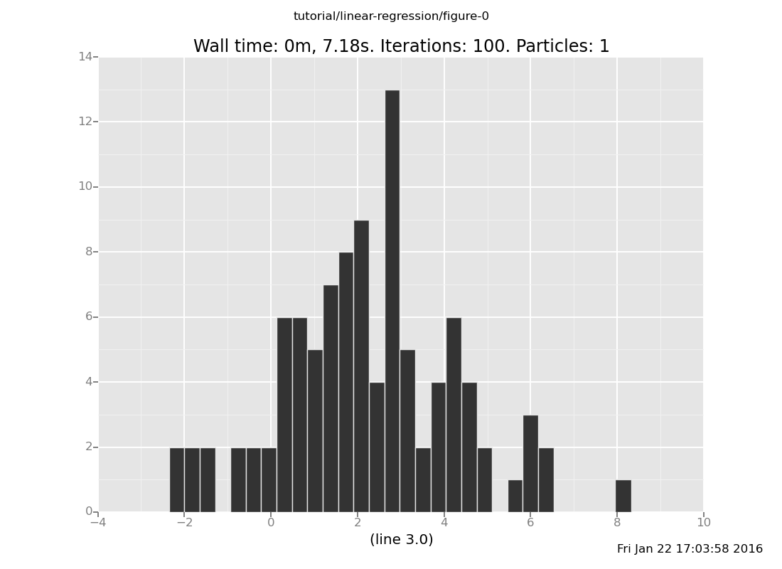
   Answer: 2, broad,

   plot("h0", data)
   

   []

   

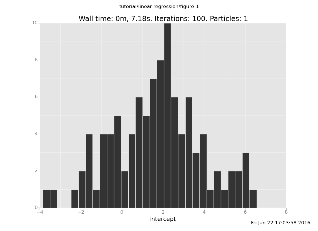
   b. Where do you expect the slope to be located, and how concentrated do you expect it to be? Plot the slope and check your intuition. (show answer)

   Answer: 0, broad,

   plot("h1", data)
   

   []

   

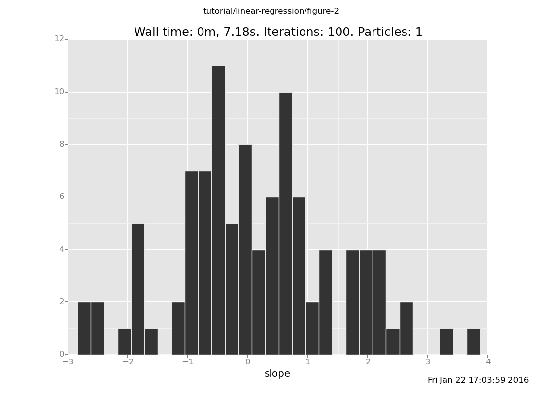
   c. What do you expect the relationship between the slope and intercept to be? Plot them against each other and check your intuition. Hint: The usual way to get a scatter plot is p0d1d: p for point and d for direct as opposed to log scale. A gotcha: if you leave the middle d off, the 0 and 1 will run together into a single index. (show answer)

   Answer: The slope and intercept are anticorrelated, because the line is trying to pass through around (1.5, 2).

   plot("p0d1d", data)
   

   []

   

Topic: Working with Datasets

In the previous segment, we started with the simple linear regression model in lin-reg-1.vnts

$ venture -f lin-reg-1.vnts --interactive

In this segment, we will try it on more data.

There is a little synthetic regression dataset in the file reg-test.csv. Download it and have a look.

You could, of course, type all this data into your Venture session as

observe obs(this) = that;
observe obs(that) = the other;
...

but that's pretty tedious. Being a probabilistic programming language, VentureScript doesn't replicate standard programming facilities like reading data files, and instead offers close integration with Python. So the way to do a job like this is to use pyexec:

run(pyexec("import pandas as pd"));
run(pyexec("frame = pd.read_csv('reg-test.csv')"));
run(pyexec("ripl.observe_dataset('obs', frame[['x','y']].values)"))

[]

list_directives

30: intercept: [assume intercept (normal 0.0 10.0)]:  2.25017975886
32: slope: [assume slope (normal 0.0 10.0)]:    -0.48478075485
34: line: [assume line (make_csp (quote (x)) (quote (add (mul slope x) intercept)))]:   <procedure>
36: obs: [assume obs (make_csp (quote (x)) (quote (normal (line x) 1.0)))]: <procedure>
38: [observe (obs 1.0) 2.0]
40: [observe (obs 2.0) 2.0]
352: [observe (obs (quote -10.0)) -1.20828529015]
353: [observe (obs (quote -9.0)) -0.567501830524]
354: [observe (obs (quote -8.0)) -0.612739408632]
355: [observe (obs (quote -7.0)) -0.354283720351]
356: [observe (obs (quote -6.0)) 0.162259994647]
357: [observe (obs (quote -5.0)) 0.680668720614]
358: [observe (obs (quote -4.0)) 1.3566224356]
359: [observe (obs (quote -3.0)) 1.31982546101]
360: [observe (obs (quote -2.0)) 1.81750436714]
361: [observe (obs (quote -1.0)) 2.16768146479]
362: [observe (obs (quote 0.0)) 3.09576830849]
363: [observe (obs (quote 1.0)) 3.02532816024]
364: [observe (obs (quote 2.0)) 2.89803542848]
365: [observe (obs (quote 3.0)) 3.29669220806]
366: [observe (obs (quote 4.0)) 4.00175073859]
367: [observe (obs (quote 5.0)) 4.44206148709]
368: [observe (obs (quote 6.0)) 4.50628393194]
369: [observe (obs (quote 7.0)) 5.13070618482]
370: [observe (obs (quote 8.0)) 5.90306800089]
371: [observe (obs (quote 9.0)) 6.00526047043]
372: [observe (obs (quote 10.0)) 6.14158080559]

If you want to know what just happened there, pyexec is an action of the inference language that executes the given string of Python code. The binding environment persists across calls, and begins with the variable ripl bound to the current session's Read-Infer-Predict Layer, which serves as the entry point for using VentureScript as a Python library. In this case, we used the escape to load our csv file up into a Pandas DataFrame, and then used the RIPL's observe_dataset method to load it into VentureScript as individual observations.

OK, so we loaded the data. We could do some inference

infer default_markov_chain(30)

[]

and ask for a prediction at a new x-value

sample line(11)

-0.0800046046182

but without a look at the data, we don't even know what to expect. There are of course plenty of ways to plot a dataset; in this case, we will use VentureScript's plot:

run(pyexec("import venture.lite.value as vv"));
define frame = run(pyeval("vv.VentureForeignBlob(frame[['x', 'y']])"));
plot("p0d1d", frame)

[]

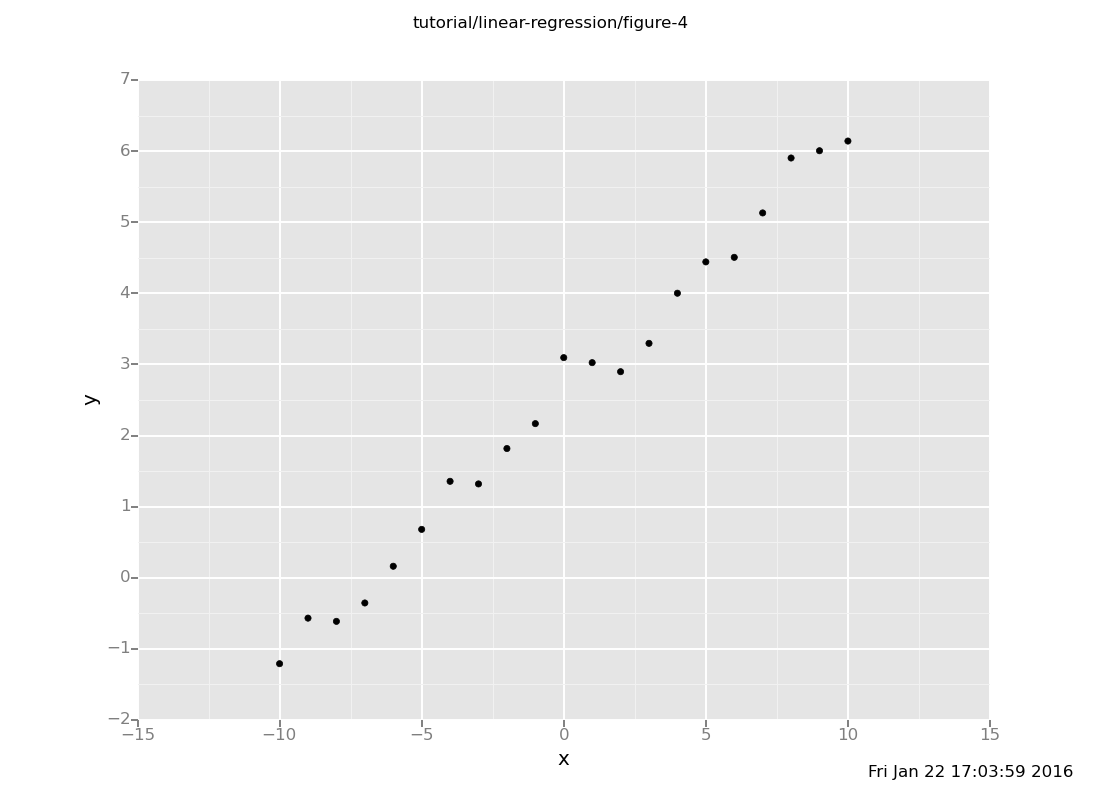
The dataset exhibits a clear linear relationship, and we should expect line(11) to be around 7.

Let's try using Markov chain inference to fit our linear model. Start 100 independent chains, evolve them for 30 iterations, and record where they end up:

define data = run(accumulate_dataset(100,
  do(reset_to_prior,
     default_markov_chain(30),
     collect(intercept, slope, line(11)))))

<venture.engine.inference.Dataset object at 0x2ae5d7367990>

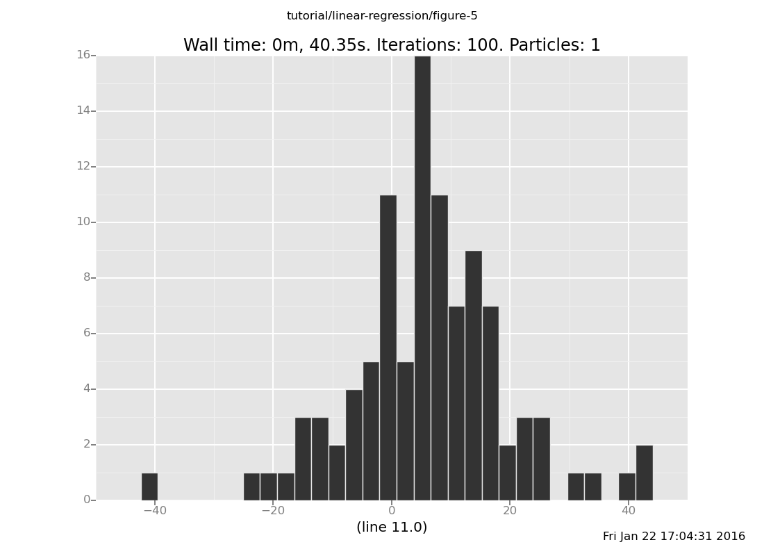
Now we can plot a histogram of the predicted line(11) value.

plot("h2", data)

[]

Topic: Understanding a model with visualization

Is our fit any good? Although we can get some idea of what's going on by plotting the predictions for a given x, it's much more effective to be able to see the fitted line plotted alongside the data, and see what happens over the course of inference.

In order to do so, we can make use of Venture's plugin infrastructure to load external code written in Python. In this case, we've provided a custom plugin that produces an animated curve-fitting visualization that can be updated during the inference program. Download curve-fitting.py and load it into VentureScript using

run(load_plugin("curve-fitting.py"))

[]

Alternatively, the plugin can be loaded when you launch Venture by supplying -L curve-fitting.py on the command line.

When the plugin loads, a new window should pop up where the animation will appear. The plugin provides a callback that can be invoked to draw a new frame

run(call_back(draw))

[]

which should render a plot that looks like this:

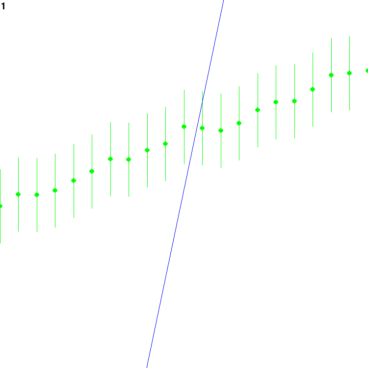
The blue line is the current guess. The green points are the observations; the error bars around them reach twice the standard deviation of the noise, above and below. The number at the top left is the count of how many frames have been drawn.

We can also plot multiple frames with inference commands interleaved

infer reset_to_prior;
infer repeat(30, do(default_markov_chain(1),
                    call_back(draw)))

[]

The repeat command works similarly to accumulate_dataset, but in this case we aren't concerned with collecting the data since it's being rendered in the visualization instead. Together, this command will run the Markov chain for 30 iterations, drawing an animation frame after each iteration.

Another useful command which works well with visualization is loop, which runs the given action continually in the background. You can use it like this

infer loop(do(default_markov_chain(5),
              call_back(draw)))

None

which will iterate the Markov chain and draw an animation frame every 5 iterations, continuing to do so indefinitely. You can turn it off with

endloop

<procedure>

Exercise: Play with this visualization to see how inference is doing.

1. Use the loop command to run the Markov chain continually and draw an animation frame after every iteration. Watch the animation while it runs and confirm that the line eventually approaches a good fit to the data. Does it take gradual steps or sudden jumps? (show answer)

   Answer: It takes sudden jumps, with varying amount of time between jumps.

   infer loop(do(default_markov_chain(1), call_back(draw)))
   

   None

2. How many iterations does it take for the chain to converge? Modify the inference loop to call reset_to_prior after every 30 iterations of the Markov chain. (Hint: You may want to use repeat and do.) Is the Markov chain able to find a good fit within 30 iterations? What about 100 iterations? Try playing with the number of iterations to see how many it takes to reliably find a reasonable fit. (show answer)

   Answer: 30 is not enough, and it may not even be obvious visually when it's resetting to the prior. 100 is better, but still often fails to find a fit; 200-300 is clearly able to find it most of the time.

   infer loop(do(reset_to_prior,
                repeat(30, do(default_markov_chain(1),
                              call_back(draw)))))
   

   None

3. (If you're still running the infer loop, turn it off for this part.)

   endloop
   

   <procedure>

   We can use resample to run multiple independent chains and plot all of the resulting lines in the same window, to get some sense of the posterior distribution over lines. Resample 20 particles (remember to reset them to the prior), run them for 30 iterations, and look at the resulting animation. Does it look like the distribution of lines converges to something plausible? If you're impatient, try increasing the number of iterations as above. (show answer)

   Answer: Some of the samples do concentrate around the correct line, but again 30 iterations is not enough to converge.

   infer resample(20);
   infer do(reset_to_prior,
           repeat(30, do(default_markov_chain(1),
                         call_back(draw))));
   infer resample(1);
   

   []

4. Inference alternatives

   a. In the optional subunit at the end of the previous chapter, we saw how to construct our own Markov chains that used custom transition operators, with a drift kernel example. Experiment with using a drift kernel for this problem. How quickly can you get it to converge by choosing a good proposal distribution? (show answer)

   Here is an example program using a Cauchy proposal kernel (you may have used something different):

   ``` define driftkernel = proc(x) { studentt(1, x, 1) };

   define driftmarkovchain = mhcorrect( onsubproblem(default, all, symmetriclocalproposal(drift_kernel)));

   infer do(resettoprior, repeat(30, do(driftmarkovchain, call_back(draw)))) ```

   []

   The Cauchy distribution has heavy tails, which means that this will usually take small steps but occasionally propose large steps. This seems to work fairly well here.

   b. As an alternative to Markov chains, we can use gradient ascent to find the best fit. Venture provides an inference primitive, grad_ascent which deterministically climbs the gradient toward the most probable parameter values. It can be invoked as follows:

   infer repeat(30, do(grad_ascent(default, all, 0.001, 1, 1), call_back(draw)))

   []

   This has a very different character than the inference primitives we've seen so far. Experiment with it, tweaking the step size (the "0.001"; be careful setting it too high!) and using reset_to_prior to start from a few different initial conditions. Can you think of some advantages and disadvantages of gradient methods compared to Monte Carlo methods? (show answer)

   Answer: Gradient ascent can move toward high-probability regions of the parameter space faster and more directly than Monte Carlo methods. However, the convergence of gradient ascent highly depends on the shape of the posterior probability density function; if the posterior density is too flat, it will move very slowly, whereas if the posterior density is too steep relative to the step size, it may overshoot and spiral off to infinity. Additionally, if there are local maxima, gradient ascent will not be able to escape them. (Markov chains are also susceptible to local maxima, although less so.)

   Convergence aside, an important conceptual difference is that gradient ascent gives only a point estimate of the single most probable values. In contrast, sampling methods return values that are (approximately) distributed according to the full posterior distribution, allowing the uncertainty in those values to be quantified and taken into account when making decisions.

Elaboration: Outlier Detection

So far, we haven't really done anything beyond what standard tools for linear least squares regression can do. Now we will look at what happens if the data may contain outliers: points that do not fit in with the rest. In ordinary least squares regression, outliers can disproportionally influence the result and so are often excluded before running the regression. Here, we will take a different approach by extending our probabilistic model to take outliers into account.

clear

We start with our linear model much the same as before

run(load_plugin("curve-fitting.py"));
assume intercept = normal(0,7);
assume slope = normal(0,4);

assume line = proc(x) { slope * x + intercept }

[]

but this time, each point has some probability of being an outlier.

assume outlier_prob = uniform_continuous(0.01,0.3);
assume is_outlier = mem(proc(i) { flip(outlier_prob) })

[]

(Here we use mem to create an indexed set of random variables is_outlier(i) for each i, which indicate whether the i-th point is an outlier.)

What does it mean for a point to be an outlier? Unlike most of the other points, which we can expect to be near the value predicted by our linear equation, an outlier could just as likely be anywhere. We will model that by saying that for an outlier point, the y-value is drawn from normal(0,20).

assume obs_outlier = proc(x) { normal(0,20) }

[]

Non-outlier points, as before, are centered on the line but subject to some Gaussian noise. This time, rather than assuming a fixed amount of noise, we will put a prior over the amount of noise as well and see how well we can infer it:

assume noise = gamma(1,1);
assume obs_inlier = proc(x) { normal(line(x), noise) }

[]

Putting that all together, our full data model is

assume obs = proc(i,x) {
  if (is_outlier(i)) {
    obs_outlier(x)
  } else {
    obs_inlier(x)
  }
}

[]

Whew. If you don't want to type all that in, it's also in lin-reg-2.vnts.

Let's try this with some data

observe obs(0,1) = 2.5;
observe obs(1,4) = 1;
observe obs(2,-3) = -1;
observe obs(3,-5) = 6

[-1277140.9512221075]

and load it into our visualization

run(load_plugin("curve-fitting.py"));
infer loop(do(default_markov_chain(1),
              call_back(draw)))

None

This should spend a while considering different hypotheses and whether or not to treat each point as an outlier. Eventually, it might find this configuration and settle on it for a while:

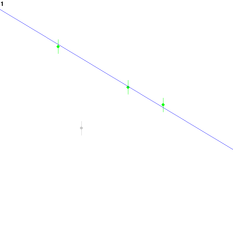
The grey dot is currently assumed to be an outlier, whereas the green ones are inliers.

endloop

<procedure>

If you are used to least squares regression, the above model may look a bit weird. A search process that was trying to minimize, say, squared error on inliers would be very happy to just call every data point an outlier and be done with it. Why doesn't the Markov chain decide to do that?

This is an instance of the phenomenon known as Bayesian Occam's Razor. On this example, it works as follows: Since we are being fully Bayesian here, we have to give a probability model for the outliers as well as the inliers. Since it's a probability model, its total mass per data point must add up to 1, just like the inlier model's total mass per data point. Since the point of the outlier model is to assign reasonable probability to a broad range of points (outliers!), it perforce cannot assign very high mass to any of them -- necessarily lower than the mass the inlier model assigns to points sufficiently near the line. Consequently, several nearly colinear points are much more likely to be inliers on a line than to all be outliers; and the Markov chain, being a correct algorithm, finds this. Philosophically, one might call the outlier model "complex", in the sense of being high entropy; and Bayesian Occam's Razor automatically causes the posterior to prefer lower entropy -- "simpler" -- explanations.

Topic: Using tags for inference control

Now that we have a more complex model with more moving parts, we'd like to be able to treat each of those parts independently when it comes to deciding how to do inference. VentureScript provides a mechanism to tag different parts of the model program and then refer to those tags from inference commands.

Let's see how this works. We'll load the same model as before, but this time we'll tag each of the random choices made in the model so that we can refer to them separately (lin-reg-3.vnts):

clear

run(load_plugin("curve-fitting.py"));
assume intercept = tag("param", "intercept", normal(0,7));
assume slope = tag("param", "slope", normal(0,4));

assume line = proc(x) { slope * x + intercept };

assume noise = tag("hyper", "noise", gamma(1, 1));

assume outlier_prob = tag("hyper", "outlier_prob", uniform_continuous(0.01, 0.3));

assume is_outlier = mem(proc(i) { tag("outlier", i, flip(outlier_prob)) });

assume obs = proc(i, x) {
  if (is_outlier(i)) {
    normal(0,20)
  } else {
    normal(line(x), noise)
  }
};

[]

Each tag command takes three arguments: a scope identifier, a block identifier, and the expression it applies to. Scope and block identifiers can be any unique expression. Inference commands can then use these identifiers to target a particular scope and block. For example, we can do Markov chain inference on just the line parameters using

infer mh("param", one, 1);

[]

The mh inference command is the same as default_markov_chain, except that it allows you to specify a scope and block to operate on; in fact, default_markov_chain(x) is an alias for mh(default, one, x). Here default is a keyword that refers to the default scope containing all random choices in the model, and one means to pick one randomly from the blocks associated with the scope.

What are scoped inference commands good for? Here are some use cases:

• Specifying how to divide effort between different parts of the model. For instance, one issue with using the default Markov chain on the model with outliers is that the default chain will consider each random choice in the model equally often, but the model contains one random choice for every data point that determines whether it's an outlier or not, so as the number of data points increases it will spend most of its time categorizing points as outliers and relatively little time actually fitting the line parameters. Using scopes, we can explicitly decide how many iterations to allocate to outlier detection to avoid having it take a disproportionate amount of effort.

• Using different inference strategies for different parts of the model. For instance, we may want to use enumerative Gibbs for the outlier detection, and drift proposals for the line parameters. This is especially useful when some inference strategies only make sense for some types of variables; in this case, enumerative Gibbs is only possible for discrete variables and normal drift proposals only make sense for continuous variables.

Let's apply these ideas to our model. Load the observations again

observe obs(0,1) = 2.5;
observe obs(1,4) = 1;
observe obs(2,-3) = -1;
observe obs(3,-5) = 6

[-3783.719945710069]

and run the following inference program:

define drift_kernel = proc(x) { student_t(1, x, 1) };

define drift_mh =
  proc(scope, block, transitions) {
    repeat(transitions,
      mh_correct(
       on_subproblem(scope, block,
         symmetric_local_proposal(drift_kernel))))
  };

infer loop(do(drift_mh("param", all, 2),
              mh("hyper", one, 1),
              gibbs("outlier", one, 1),
              call_back(draw)))

None

This will alternate between the different tagged parts of the model, using a different inference strategy for each one.

Exercise: Compare this to the infer loop that only used default_markov_chain from earlier. What qualitative differences in behavior do you see? Try adjusting the number of iterations allocated to each scope and see what happens. (show answer)

Exercise: What happens if you replace drift_mh with grad_ascent? Hint: Make sure to pass the appropriate scope and block to grad_ascent. (show answer)

infer loop(do(grad_ascent("param", all, 0.001, 10, 1),
              mh("hyper", one, 1),
              gibbs("outlier", one, 1),
              call_back(draw)))

None

endloop

<procedure>