| < Prev: Top | ^ Top | Next: More VentureScript: Linear Regression > |
In this chaper, we will go through the basic, foundational concepts in VentureScript: sampling, models, and automatic inference. The practice model will intentionally be very simple, so that it's possible to understand very clearly what's happening.
Start a Venture session by running
$ venture
venture[script] >This command starts an interactive interpreter for VentureScript. In general, this tutorial will show interactions in grey blocks as above, with the user input in roman font, and the system's output in italics.
You can also run VentureScript scripts by making a file with a .vnts
extension and running
$ venture -f script.vnts
N.B.: The command line reference
explains what's happening here and what other options venture accepts.
Sample an expression
uniform_continuous(0, 1)
0.405929869128These are independent samples from the unit uniform distribution
uniform_continuous(0, 1)
0.919535130201We can introduce a variable:
define mu = expon(2) // Exponential distribution with rate 2
0.435758525422whose value is a particular sample from that distribution:
mu
0.435758525422and we can sample further expressions conditioned on that value:
normal(mu, 0.2)
0.137322063299Exercise: Convince yourself that, for any given mu, normal(mu, 0.2)
is a different distribution from
normal(expon(2), 0.2)
0.594927537869because the latter samples a new internal mu every time. Drawing just a few samples from each should suffice.
You can find the list of distributions (and deterministic functions) available in VentureScript in the appropriate section of the reference manual.
Now clear your session (or quit and restart Venture) for the next segment:
clear
When we used define to make a mu variable in the previous
segment, that variable's value was fixed to a particular sample from
its generating distribution for the remainder of the program.
In order to make variables that we can learn things about by
observation and reasoning, we need to flag them as uncertain, using
assume:
assume x = normal(0, 1)
0.77582238738Now x is a normally distributed random variable, and its current
value is a sample from that distribution.
Assumed and defined variables live in separate namespaces in
VentureScript: define goes into the toplevel namespace,
and assume goes in the model namespace. Bare expressions
are evaluated in the toplevel namespace, so just typing x gives an error:
x
*** evaluation: Cannot find symbol 'x'
(autorun x)
         ^
To access the current value of an assumed variable, we use sample
sample x
0.77582238738because sample runs its expression in the model namespace (without
altering the content of the model).
Note that repeated access to x gives the same value each time:
sample x + x
1.55164477476That's what allows us to form models with conditional dependencies, such as this extension:
assume y = normal(x, 1)
1.2123631843So, why is assume any more useful than define? Models, unlike the
top level, allow us to register observations:
observe y = 2
[-1.6682439468250236]sample y
2.0Note: the value of x doesn't change yet --
sample x
0.77582238738-- all we did was register an observation.
Now infer.
infer conditional
[]Now x is a sample from the conditional distribution p(x|y=2) defined
by our assumptions and observations:
sample x
1.08482866678If we do no more inference, x doesn't change.
sample x
1.08482866678But we can compute a new conditional sample by running the conditional inferrer again.
infer conditional;
sample x
-0.346803499748As a reminder, we were studying this model (you can skip this block if you have your session from the last segment):
clear;
assume x = normal(0, 1);
assume y = normal(x, 1);
observe y = 2
[-4.587739463361579]We can get samples from inference
infer conditional;
sample x
1.31562710058but are they actually from the right distribution? We could eyeball it like this a bit more:
infer conditional;
sample x
1.4087344761infer conditional;
sample x
1.7701375461but that will get old quickly.
It's better to gather data programmatically, for example like this:
define data = run(accumulate_dataset(10, do(conditional, collect(x))))
<venture.engine.inference.Dataset object at 0x2b673f956850>If you really want to know what's going on in this expression you can
study the documentation of do, run, accumulate_dataset, and collect. The effect is to gather up the
values of x (and some metadata) over 10
iterations of the conditional inference command.
print(data)
   iter  prt. id  time (s)  log score  prt. log wgt.  prt. prob.         x
0     1        0  0.025771  -3.408019      -4.587739           1  0.244922
1     2        0  0.028528  -3.658097      -4.587739           1  1.905660
2     3        0  0.030490  -2.905525      -4.587739           1  1.260092
3     4        0  0.032223  -3.408832      -4.587739           1  1.755615
4     5        0  0.034123  -2.887258      -4.587739           1  0.777781
5     6        0  0.037368  -3.043581      -4.587739           1  1.453546
6     7        0  0.040359  -2.994216      -4.587739           1  0.604603
7     8        0  0.042707  -2.999298      -4.587739           1  0.598228
8     9        0  0.044609  -2.924843      -4.587739           1  0.705100
9    10        0  0.047014  -3.783363      -4.587739           1  1.972361

[10 rows x 7 columns]
[]Do those values of x look good? The values look sane to me, but I
can't eyeball a table of numbers and tell whether they are distributed
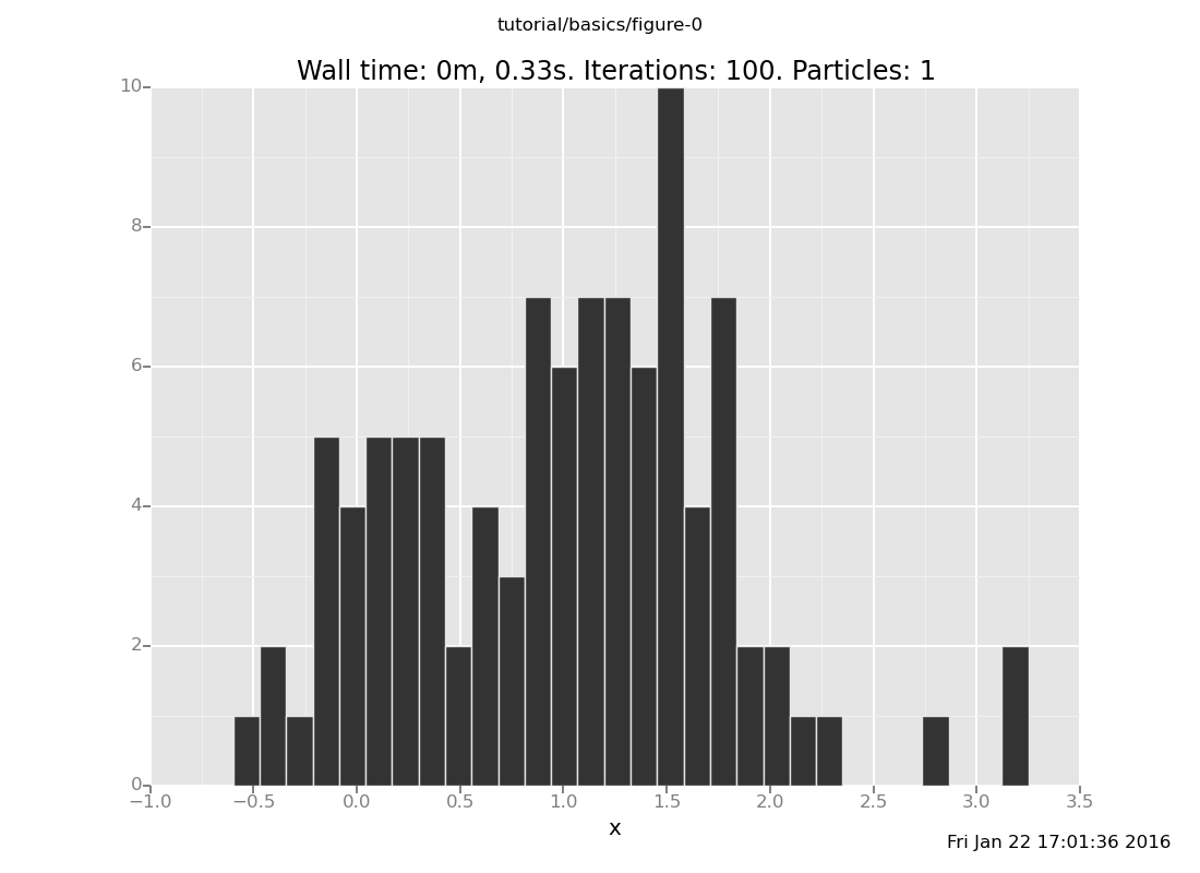
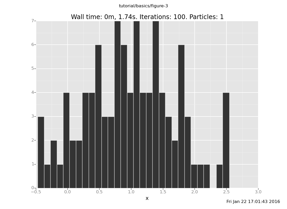
properly. Let's get more data and plot it:
define more_data = run(accumulate_dataset(100, do(conditional, collect(x))))
<venture.engine.inference.Dataset object at 0x2b673f9ba510>plot("h0", more_data)
[]
That h0 says "make a histogram of the zeroth collected data stream".
You will eventually want to study the plot spec reference,
because that explains how to plot any of the values or metadata collected in the dataset
on the x, y, or color axis of a plot.
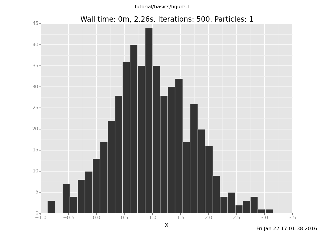
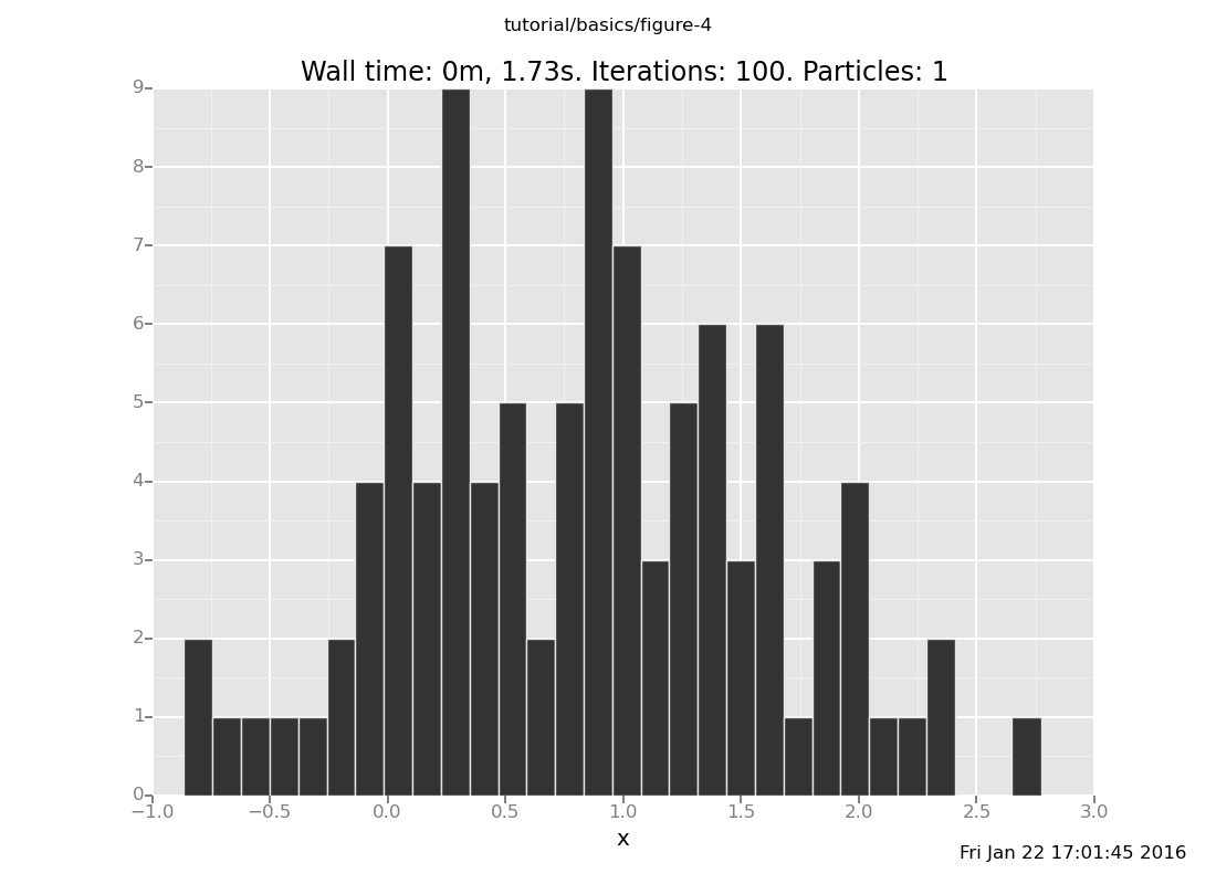
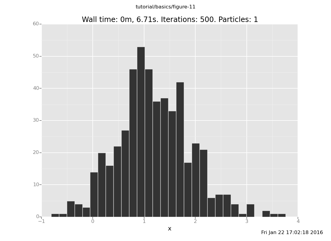
Here's a version with more samples for better resolution:
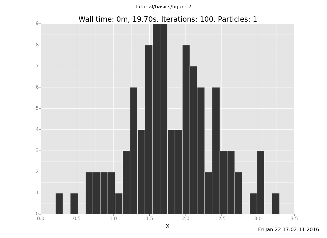
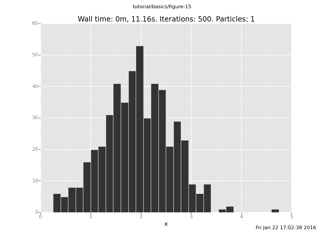
plot("h0", run(accumulate_dataset(500, do(conditional, collect(x)))))
[]
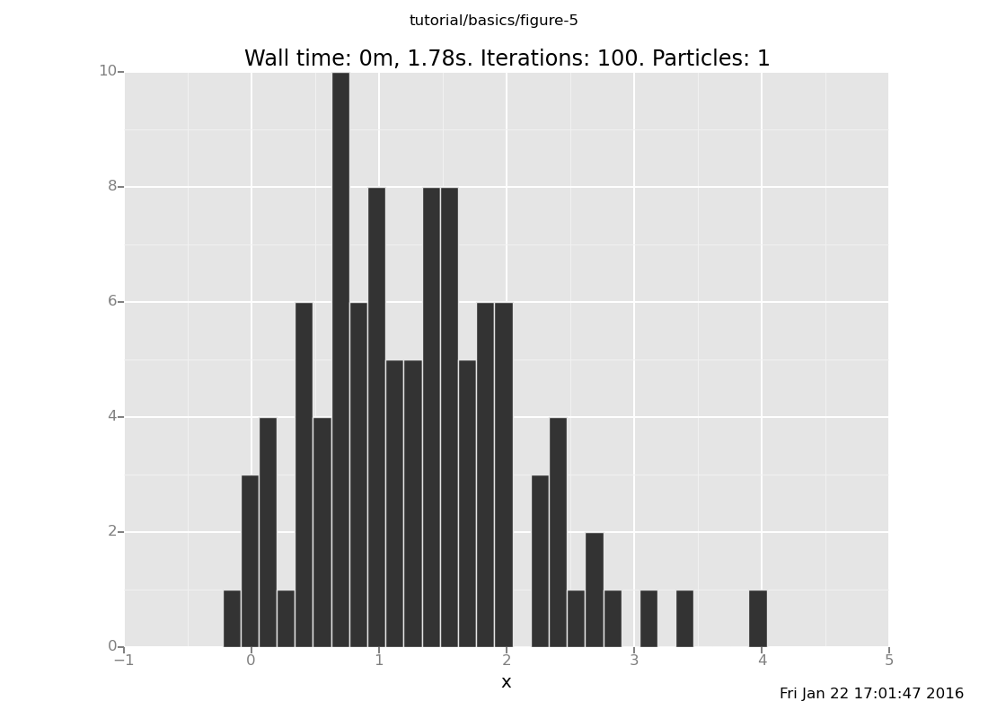
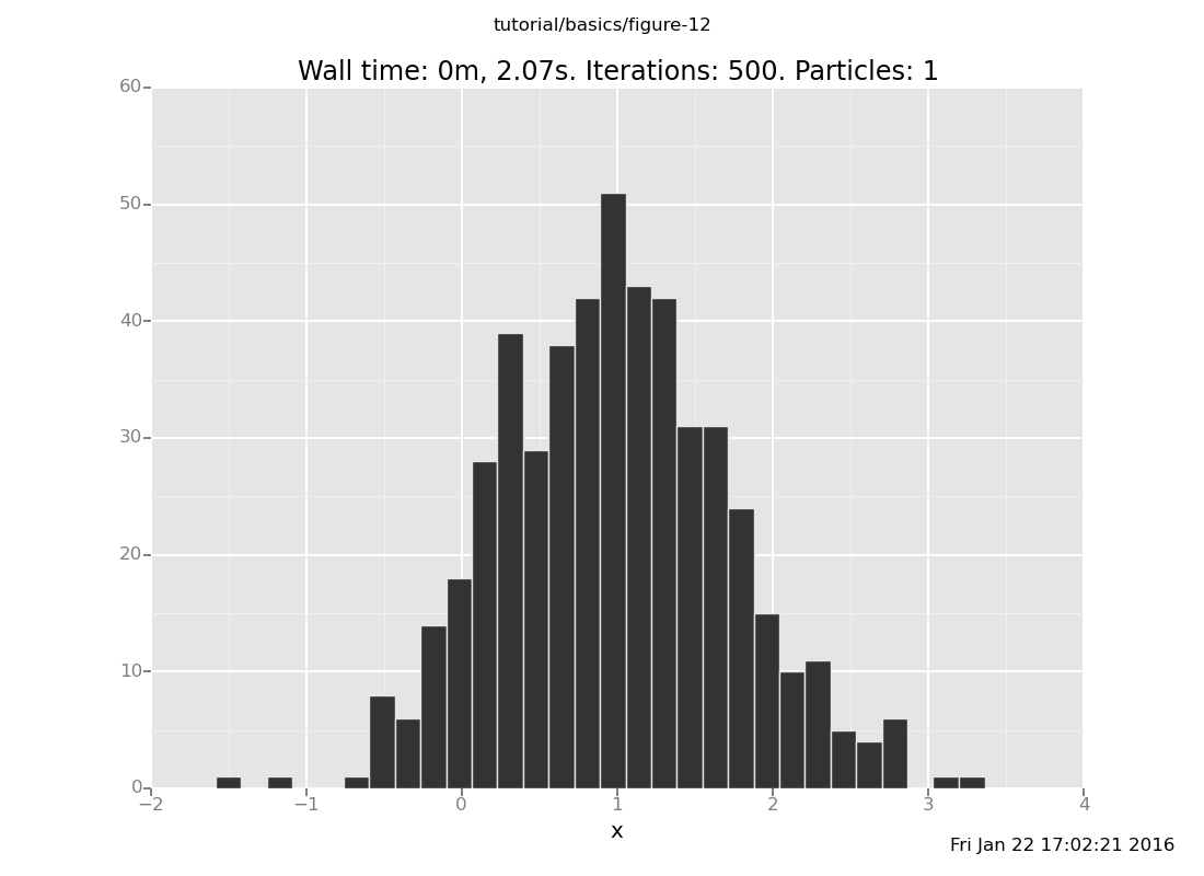
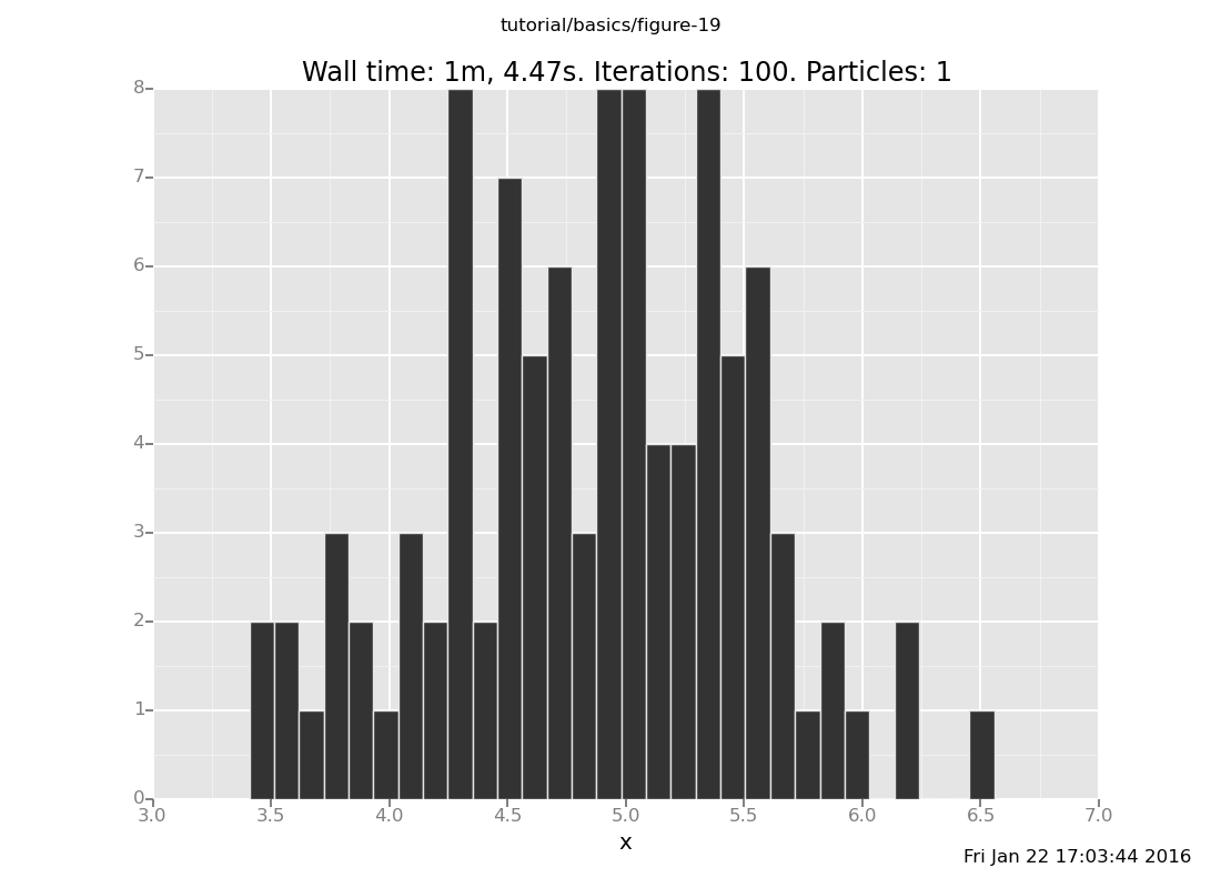
The analytical answer is a Gaussian with mean 1 and precision 2 (which
is standard deviation 1/sqrt(2)), whose histogram looks like this:
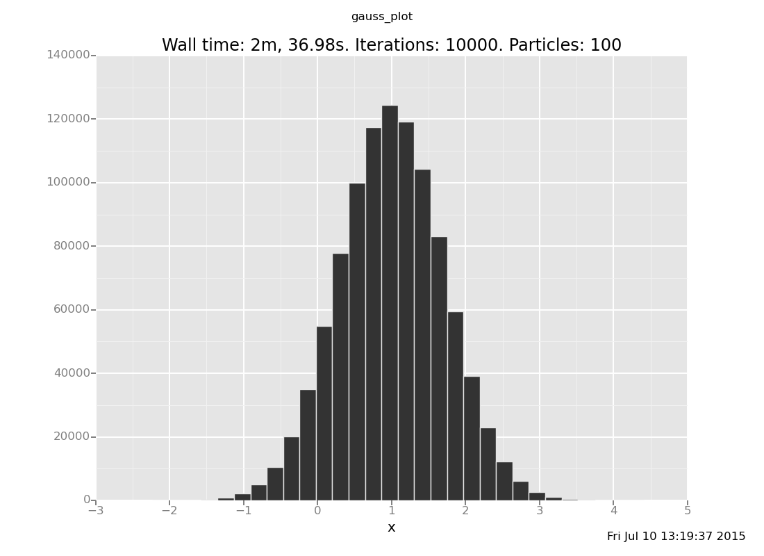
Exercise: How visually close can you get to this plot by increasing the number of iterations (the 500) in the above expression? Is inference working? Are you satisfied with how fast it is?
In the next segment, we will look at a few different inference strategies, which give different speed-accuracy tradeoffs.
In this segment, we will look at a few different generic inference strategies that are built in to VentureScript and do some basic exploration of their speed-accuracy behavior. As a reminder, here is the model we are working with (you can skip this block if you have your session from the last segment):
clear;
assume x = normal(0, 1);
assume y = normal(x, 1);
observe y = 2
[-1.8541841367539602]If you're curious why we're looking at the performance of inference on such a simple model, there are a couple reasons:
There is an analytic solution, which means the correct result is available for comparison.
The Gaussian distribution is actually a pretty good proxy for general probability problems: the mean corresponds to "the true result" and the standard deviation corresponds to "the uncertainty" or "the error tolerance".
The position of the observation is a proxy for the "difficulty" of the problem: the further out the data are from the prior, the more inference needs to overcome in order to reach the right answer.
The one down side is that this problem in one-dimensional, so you need to exercise active skepticism around your geometric intuitions: try and cross-check the mental pictures you build for how they would work in 2, 3, 10, or 10,000 dimensions.
The inference command conditional is global rejection sampling -- guessing and checking. As you might know or imagine, this is likely to get slow. In particular, let's fiddle with the position of the observation and see what happens as we change the model to make the problem harder.
If you like standalone scripts, save the following into a file named,
say, exact.vnts
assume x = normal(0, 1);
assume y = normal(x, 1);
observe y = 2;
plot("h0",
 run(
  accumulate_dataset(100,
   do(conditional,
      collect(x)))))
and explore by editing it and rerunning it with
$ venture -f exact.vnts
If you prefer to fiddle interactively, VentureScript has a command named
forget for removing parts of a model so they can be changed.
First, check what's in the model already:
list_directives
30: x: [assume x (normal 0.0 1.0)]:   0.632340975572
32: y: [assume y (normal x 1.0)]:   2.0
34: [observe y 2.0]
[Note: The above output is presented in a prefix notation syntax that represents how VentureScript actually parsed it.]
Then use forget to remove the existing observation, and replace it
with one where the datum is farther out.
forget(34);
observe normal(x,1) = 4
[-6.589502185609396]list_directives
30: x: [assume x (normal 0.0 1.0)]:   0.632340975572
32: y: [assume y (normal x 1.0)]:   2.0
37: [observe (normal x 1.0) 4.0]
The same solution still works
plot("h0", run(accumulate_dataset(100, do(conditional, collect(x)))))
[]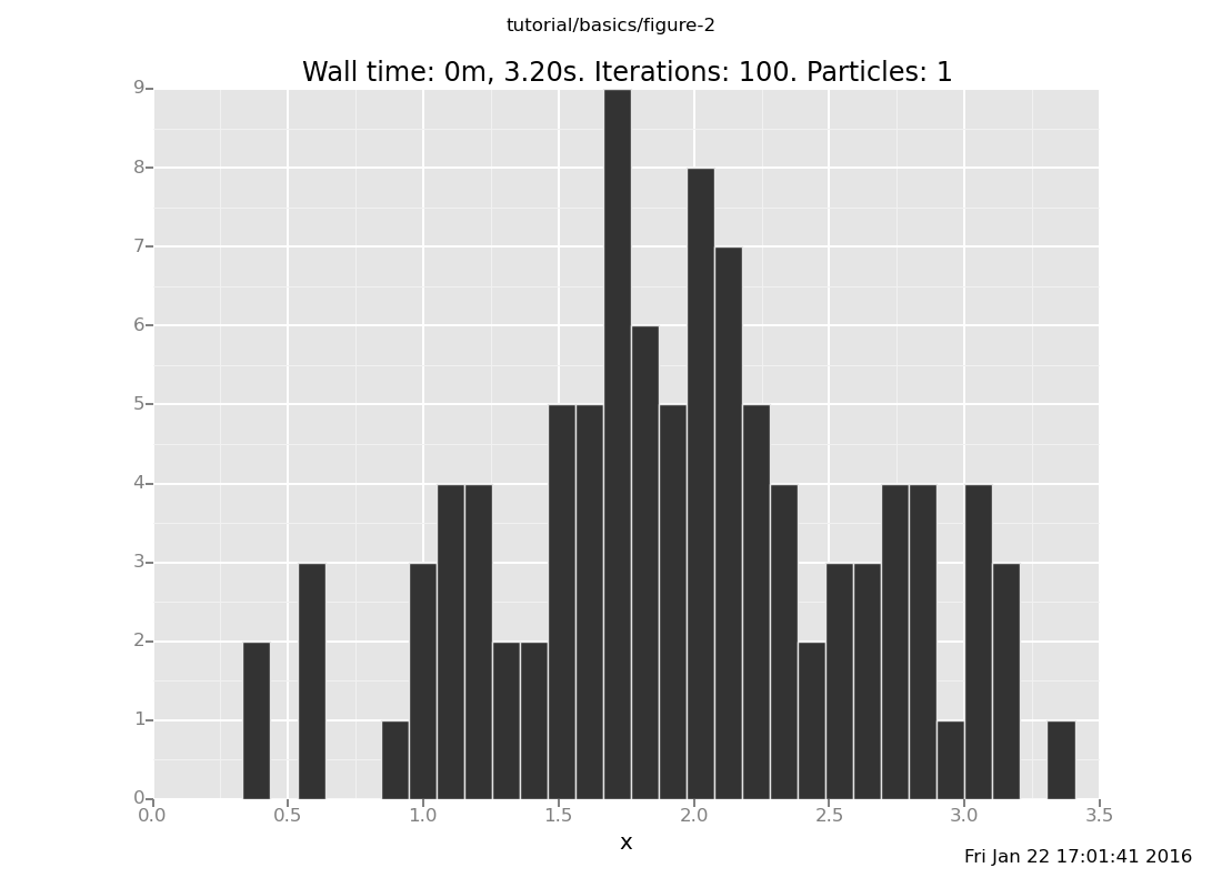
but as you move the datum still further out (with more forget and
observe commands), you can tell that more distant observations take
longer to get samples for. Don't move the datum too far: rejection takes
e^(O(position^2)) time on this problem.
The inference phenomenon at work here is this:
The KL divergence from the conditional (e.g. posterior) to the marginal (e.g. prior) is one notion of the "distance" between the conditional and the marginal. Intuitively, we can think of this KL divergence as measuring the difficulty of the problem. In the current example, the KL divergence grows quadratically with position of the datum.
Rejection sampling (which is the algorithm the conditional command
uses) is exponentially slow in the KL gap it is trying to
cross. This is one
case in which the intuitive notion that KL divergence measures the difficulty
of inference has been made precise.
A very common inference technique is importance sampling with resampling. It is:
Draw some number of trials (or "particles") from the prior [or any proposal distribution of your choice]
Weight them by the likelihood [or the ratio between the posterior and proposal probabilities]
Select one at random in proportion to its weight [or more than one, but then they are not independent of each other]
Here's what a basic version of this looks like in VentureScript. Reset the model if you need to
clear;
assume x = normal(0, 1);
assume y = normal(x, 1);
observe y = 4
[-2.8683745957235502]or load your file from the rejection segment into an interactive session with
venture -f exact.vnts -i
Then make 5 particles
infer resample(5)
[]The resample inference action makes as many particles as requested by drawing from the existing pool proportionally to their weight, and then makes the weights equal (this compound operation is very common in sequential Monte Carlo or particle filter methods). Initially there is just one particle, so right now all of them are the same:
run(sample_all(x))
[2.025443815679646, 2.025443815679646, 2.025443815679646, 2.025443815679646, 2.025443815679646]To do importance sampling, we next reset them to the prior and weight by likelihood:
infer likelihood_weight();
run(sample_all(x))
[-0.8955055878983408, -2.1021938017714907, 0.46228089851610266, -0.4621024509220127, 0.4478408182890418]and then resample down to one, which picks a particle at random in proportion to its weight.
infer resample(1);
sample x
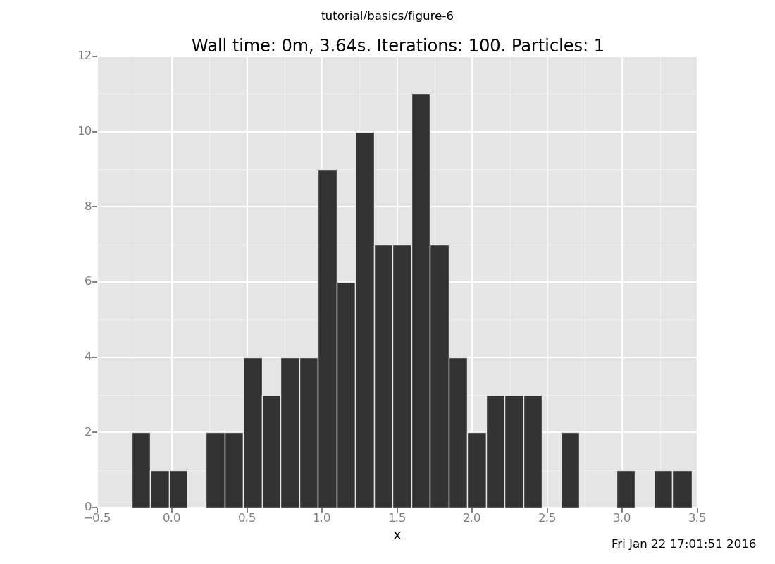
0.447840818289Using the plotting tools we learned before, here's the distribution
this algorithm makes (note the use of do to sequence inference actions):
plot("h0", run(accumulate_dataset(100,
  do(resample(5),
     likelihood_weight(),
     resample(1),
     collect(x)))))
[]
What is going on here? If you put the observation at 4, then the answer should be a Gaussian with mean 2, but the distribution with 5 trials is not even close (though it has moved from the prior). This is our first approximate inference algorithm, and generates our first time-accuracy tradeoff.
Exercises:
Vary the location of the observation without varying the inference program. Confirm that the runtime does not change, but the quality of the result (relative to the true posterior) does. (show answer)
Answer: With the observation at y = 2
clear;
assume x = normal(0, 1);
assume y = normal(x, 1);
observe y = 2;
plot("h0", run(accumulate_dataset(100,
  do(resample(5),
     likelihood_weight(),
     resample(1),
     collect(x)))))
[]
and at y = 6
clear;
assume x = normal(0, 1);
assume y = normal(x, 1);
observe y = 6;
plot("h0", run(accumulate_dataset(100,
  do(resample(5),
     likelihood_weight(),
     resample(1),
     collect(x)))))
[]
Vary the number of trials (the argument to the first resample) for a fixed location of the datum. Confirm that the runtime is asymptotically linear in that, and that the result distribution approaches the true posterior as the number of trials increases. (show answer)
Answer: With 10 trials
clear;
assume x = normal(0, 1);
assume y = normal(x, 1);
observe y = 4;
plot("h0", run(accumulate_dataset(100,
  do(resample(10),
     likelihood_weight(),
     resample(1),
     collect(x)))))
[]
and with 50 trials
clear;
assume x = normal(0, 1);
assume y = normal(x, 1);
observe y = 4;
plot("h0", run(accumulate_dataset(100,
  do(resample(50),
     likelihood_weight(),
     resample(1),
     collect(x)))))
[]
What happens if we don't do the second resample at all? Why?
(show answer)
Answer: We get samples from the prior, because we are not using the weights.
What happens if we draw more than 1 particle in the second
resample? Why?
(show answer)
Answer: This is more subtle.
Both rejection sampling and importance sampling consist of guessing possible explanations of the data, without taking advantage of previous guesses when forming new ones. The other major class of inference algorithms tries to take advantage of what has already been learned by retaining a "current state" and (stochastically) evolving it by trying various adjustments in some way arranged to approach the posterior in distribution. Broadly, such algorithms are called Markov chains. (The Markovness is that the "current state" holds all the information about the chain's history that is relevant to determining its future evolution.)
VentureScript has extensive facilities for constructing Markov chain inference strategies. In this segment, we will explore the behavior of a simple generic one on the single-variable normal-normal problem we have been studying.
Reset the model if you need to
clear;
assume x = normal(0, 1);
assume y = normal(x, 1);
observe y = 4;
sample x
0.441768072702The inference command default_markov_chain(1) takes one step of
VentureScript's default Markov chain, possibly changing the value of x.
infer default_markov_chain(1);
sample x
0.441768072702If we do that a few more times,
infer default_markov_chain(1);
sample x
0.441768072702infer default_markov_chain(1);
sample x
0.441768072702infer default_markov_chain(1);
sample x
0.441768072702infer default_markov_chain(1);
sample x
0.441768072702we should see x moving (perhaps haltingly and non-monotonically)
toward regions of high posterior mass.
(Aside: Internally, Venture's default Markov chain uses an instance of an algorithm template called Metropolis-Hastings, which examines random choices made during the program execution, samples new proposed values for those choices, and decides whether to accept a proposed value based on a ratio of likelihoods.)
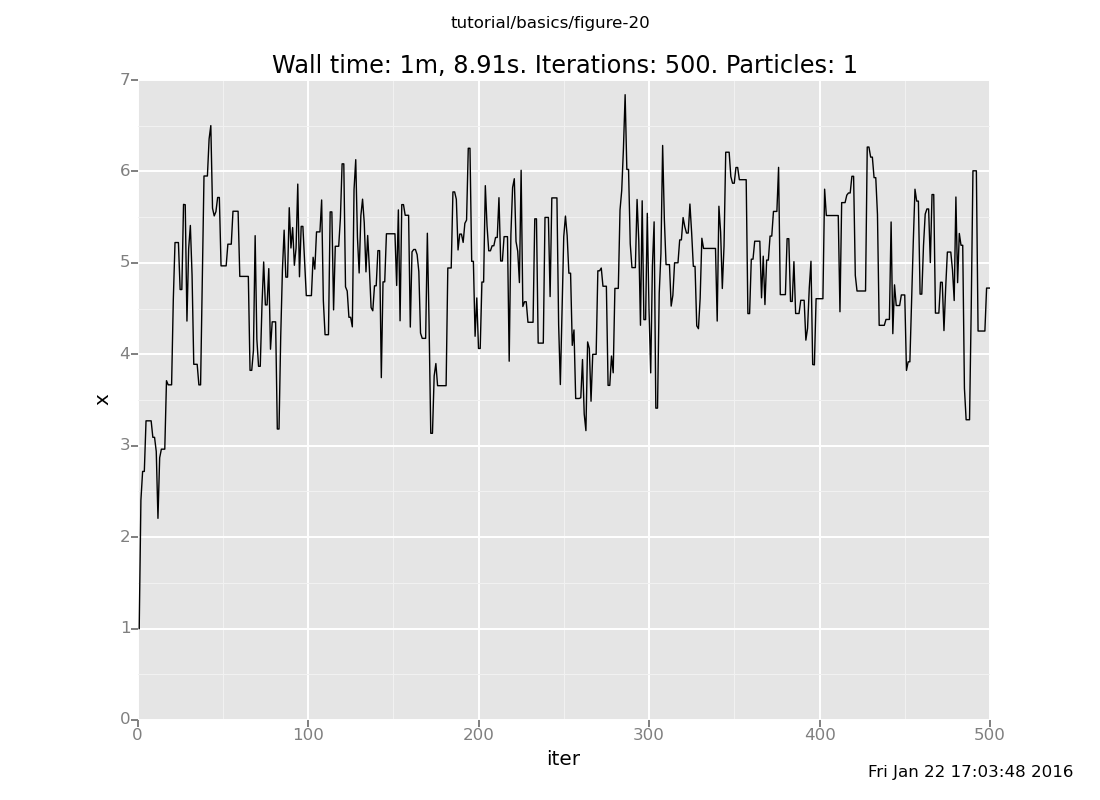
As usual, let's see that with more data:
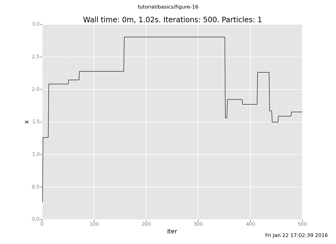
define chain_history = run(accumulate_dataset(500, do(default_markov_chain(1), collect(x))))
<venture.engine.inference.Dataset object at 0x2b67480e0710>plot("lc0", chain_history)
[]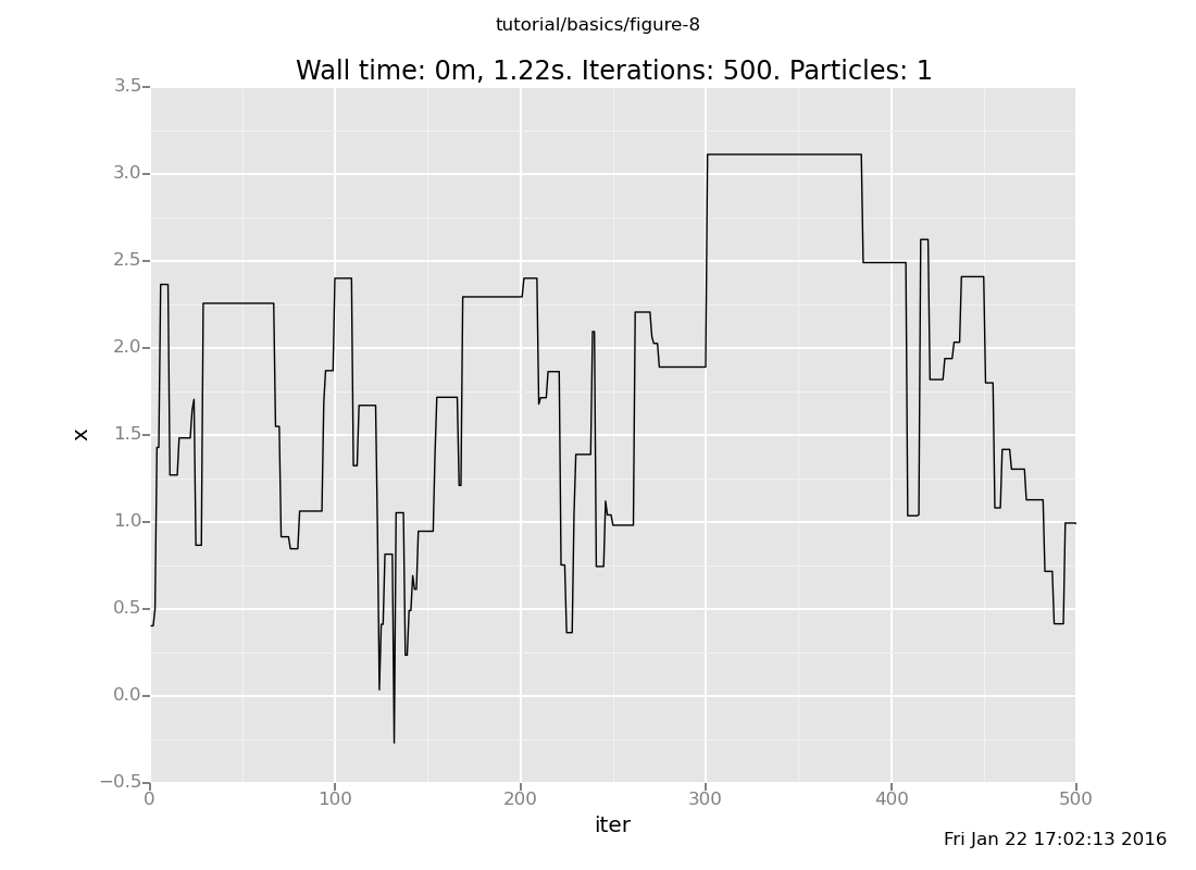
The lc0 says "make a line plot of the 0th collected expression vs
the iteration count"; here's the reference.
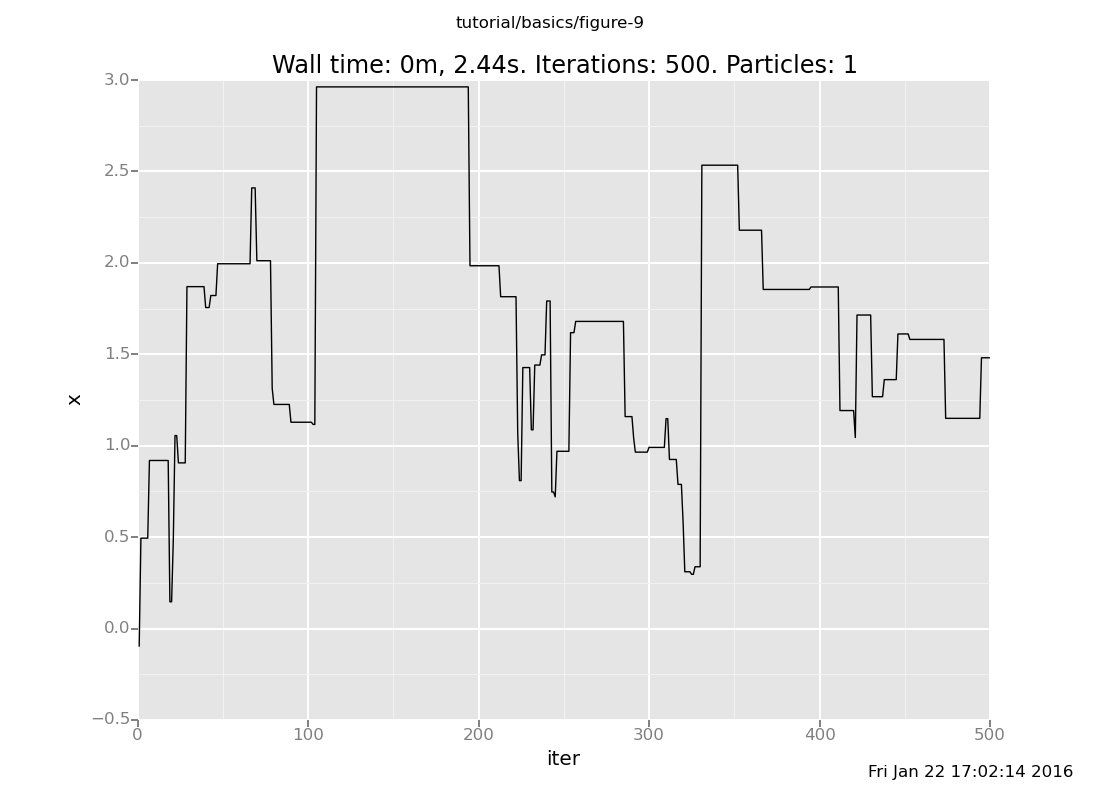
That was one particular chain. Let's see how their histories vary. First reset the state to the prior
infer reset_to_prior
[]and let's plot another one:
plot("lc0", run(accumulate_dataset(500, do(default_markov_chain(1), collect(x)))))
[]
For more insight, let's plot several independent chains together. If
we don't use the weights for anything, VentureScript's particles will serve
to run several independent chains (the r in the plot specification
means color the lines by particle id).
infer resample(20);
infer reset_to_prior;  // Reset after resampling to get independent initialization
plot("lc0r", run(accumulate_dataset(100, do(default_markov_chain(1), collect(x)))))
[]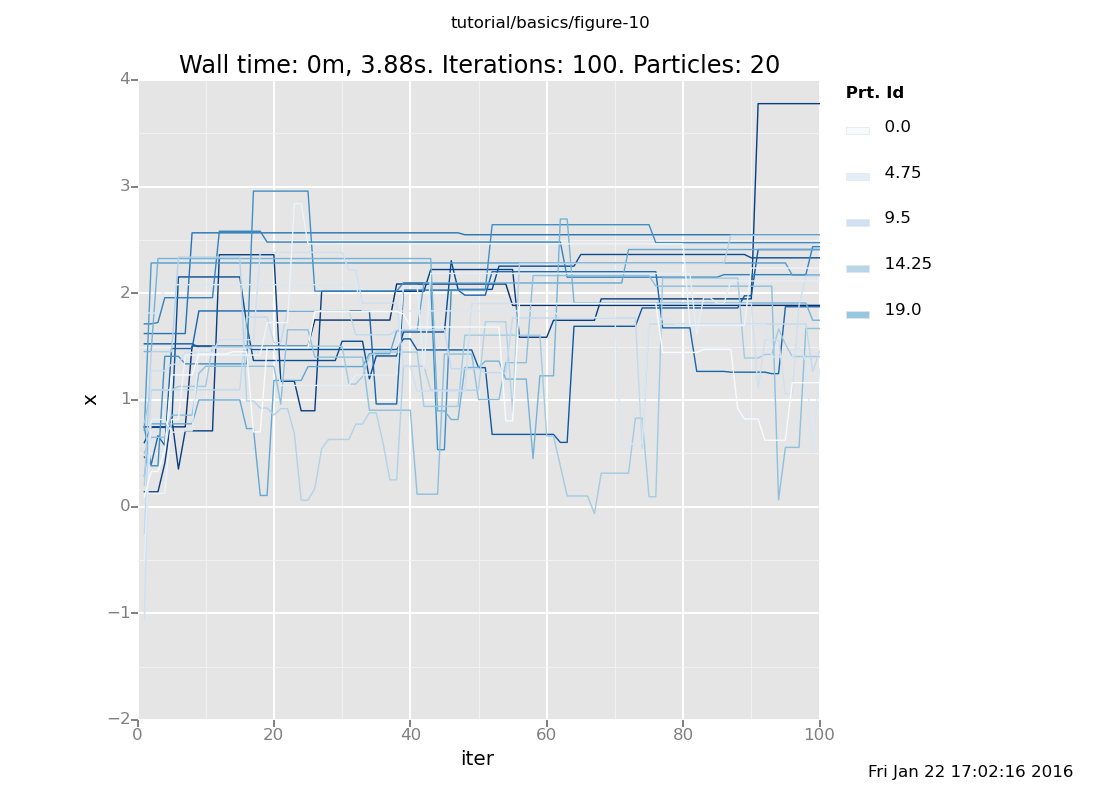
That gives a flavor for how the chains evolve to compute a solution to this problem. We can also more precisely characterize the distribution that obtains after taking some number of steps by plotting the end point rather than the history
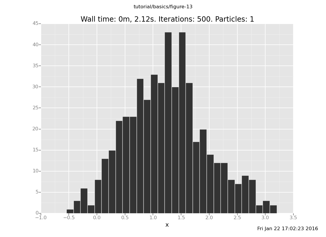
infer resample(1);  // Back to 1 particle
plot("h0", run(accumulate_dataset(500,
   do(reset_to_prior,
      default_markov_chain(5),
      collect(x)))))
[]
Notice that a 5-step chain does not suffice, on this problem, to get to the right answer in distribution. This our second approximation algorithm.
Exercises:
Vary the location of the observation without varying the inference program. Confirm that the runtime of a fixed-length chain does not change, but the quality of the result (relative to the true posterior) does. (show answer)
Answer: With the observation at y = 2
clear;
assume x = normal(0, 1);
assume y = normal(x, 1);
observe y = 2;
plot("h0", run(accumulate_dataset(500,
  do(reset_to_prior,
     default_markov_chain(5),
     collect(x)))))
[]
and at y = 6
clear;
assume x = normal(0, 1);
assume y = normal(x, 1);
observe y = 6;
plot("h0", run(accumulate_dataset(500,
  do(reset_to_prior,
     default_markov_chain(5),
     collect(x)))))
[]
Vary the number of transitions for a fixed location of the datum. Confirm that the runtime is asymptotically linear in that, and that the result distribution approaches the true posterior as the number of steps increases. (show answer)
Answer: With 10 transitions
clear;
assume x = normal(0, 1);
assume y = normal(x, 1);
observe y = 4;
plot("h0", run(accumulate_dataset(500,
  do(reset_to_prior,
     default_markov_chain(10),
     collect(x)))))
[]
and with 50 transitions
clear;
assume x = normal(0, 1);
assume y = normal(x, 1);
observe y = 4;
plot("h0", run(accumulate_dataset(500,
  do(reset_to_prior,
     default_markov_chain(50),
     collect(x)))))
[]
What happens if we don't reset_to_prior?
(show answer)
Answer: Now the histogram includes successive states of one long Markov chain. Most of those data points will be individually distributed according to the posterior, but if the number of steps between them is too small, they will not be independent.
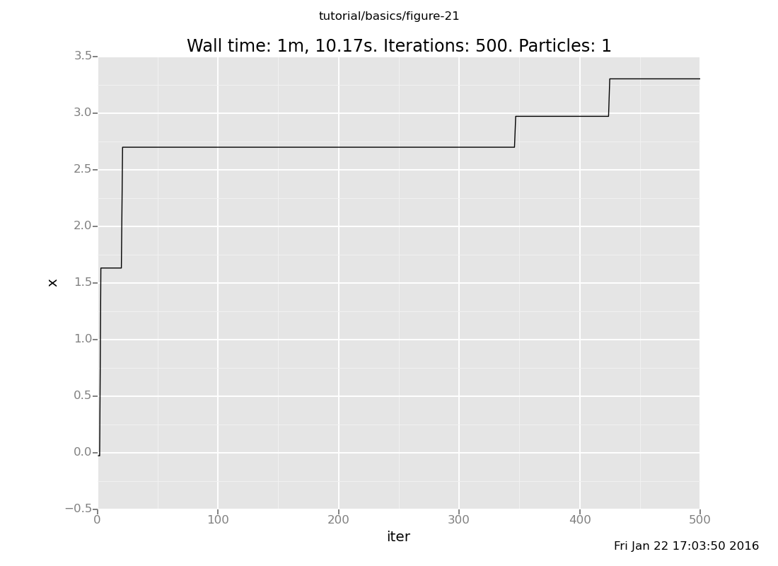
Increase both the location of the observation (making the problem harder) and the number of transitions (doing more work). How fast does the latter have to move to keep up with the former? What does the history of a long chain on a hard observation look like? (show answer)
Answer: The further the chain gets, the longer it will sit still before advancing.
clear;
assume x = normal(0, 1);
assume y = normal(x, 1);
observe y = 6;
plot("lc0", run(accumulate_dataset(500, do(default_markov_chain(1), collect(x)))))
[]
The reason this happens is that the default Markov chain proposes new candidate values from the prior, independently of the current state. If most of the prior mass has lower posterior probability than the current state, the chain will only rarely make progress. In this case, the probability of proposing a new state larger than the current one decreases exponentially, but at least it's not the squared exponential of rejection sampling.
Although the default Markov chain works well for a number of problems, and is noticeably more tractable than rejection sampling, it still suffers from the problem that it has difficulty proposing good moves when the posterior is far from the prior (see the last exercise in the previous section).
One approach that can improve performance on these problems is to take
advantage of the fact that the current state of the Markov chain is
probably better than an average sample from the prior. This suggests
that a Markov chain that proposes transitions that are close to the
current state may do better than one that proposes from the prior
every time (as default_markov_chain does).
VentureScript has an experimental library of procedures for constructing Metropolis-Hastings proposals from user-supplied transition functions. The proposals generated by these procedures are automatically weighted in favor of more probable values so that the resulting Markov chain is probabilistically correct, in that it targets the true posterior as its stationary distribution.
We can use these features to implement custom Markov chain inference strategies. Let's revisit our model once again, this time with the observation quite far away from 0:
clear;
assume x = normal(0, 1);
assume y = normal(x, 1);
observe y = 10;
[-52.47153760188347]Since the observation is so far from the prior, default_markov_chain
will have a hard time drawing an x from the prior that is more
likely than its current value. Instead, let's have our Markov chain
propose values that are centered around the current value of x:
define drift_kernel = proc(x) { normal(x, 1) };

define my_markov_chain =
  mh_correct(
   on_subproblem(default, all,
     symmetric_local_proposal(drift_kernel)));
{'fields': (<venture.lite.sp.VentureSPRecord object at 0x2b67468210d0>,), 'tag': 'inference_action', 'type': 'record'}The important part of the above code snippet is drift_kernel, which
is where we say that at each step of our Markov chain, we'd like to
propose a transition by sampling a new state from a unit normal
distribution whose mean is the current state. The rest of the code is
scaffolding that applies the Metropolis-Hastings correction and turns
it into an inference action that we can run; if you'd like to
understand it in detail, refer to the documentation of
mh_correct,
on_subproblem, and
symmetric_local_proposal.
Let's give our new Markov chain a whirl:
infer my_markov_chain;
sample x
-0.154072982668infer my_markov_chain;
sample x
0.242785879301infer repeat(10, my_markov_chain);
sample x
2.62918869553Looks promising... now let's plot the distribution it makes, as we have been doing:
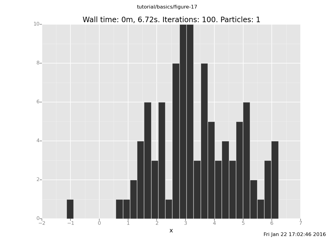
plot("h0", run(accumulate_dataset(100,
   do(reset_to_prior,
      repeat(10, my_markov_chain),
      collect(x)))));
[]
Exercises:
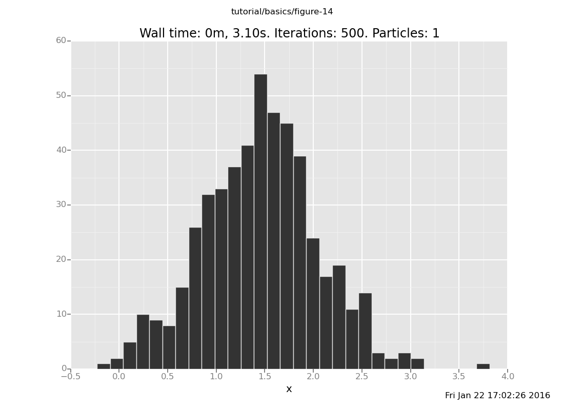
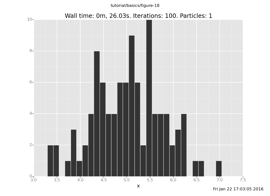
Vary the number of transitions in the above plot command. How many
transitions does it take for the result distribution to get
reasonably close to the posterior (which should be centered around
5 with standard deviation 1/sqrt(2))?
Answer: Shown below are plots after 30 and 60 transitions, respectively, which suggest that the chain has basically converged after 30 transitions.
plot("h0", run(accumulate_dataset(100,
  do(reset_to_prior,
     repeat(30, my_markov_chain),
     collect(x)))));
[]
plot("h0", run(accumulate_dataset(100,
  do(reset_to_prior,
     repeat(60, my_markov_chain),
     collect(x)))));
[]
Run a few independent chains for 500 transitions and plot the chain
histories. Compare this with 500 transitions of the
default Markov chain. (Remember to reset_to_prior before each of
these.) Which one is more effective at moving toward and exploring
the posterior?
(show answer)
Answer: Here is our Markov chain
infer reset_to_prior;
plot("lc0", run(accumulate_dataset(500, do(my_markov_chain, collect(x)))))
[]
and here is default_markov_chain:
infer reset_to_prior;
plot("lc0", run(accumulate_dataset(500, do(default_markov_chain(1), collect(x)))))
[]
Notice that our Markov chain finds the posterior much more quickly and accepts many more transitions, while the default chain gets stuck for long periods of time without moving.
Can you think of any downsides of this approach? (Hint: are there any types of posterior distributions that might give it trouble?) (show answer)
Answer: If the posterior has multiple modes, drift proposals will tend to get stuck in one of the modes, since transitioning from one mode to another requires making a large step.
(Open-ended) Experiment with different transition kernels. What
happens if you adjust the variance of drift_kernel? What if
instead of a normal distribution you use a uniform distribution
centered around the current state, or a heavy-tailed distribution
like Student's t distribution? (Hint: uniform_continuous, student_t. Note that if you redefine
drift_kernel, you'll have to re-paste the definition of
my_markov_chain above.)
| < Prev: Top | ^ Top | Next: More VentureScript: Linear Regression > |