| < Prev: More VentureScript: Linear Regression | ^ Top |
In this chapter, we will take a dive into some more advanced modeling idioms. We will move faster than we did in previous chapters. You can skim this for a flavor of the sorts of things that are possible in VentureScript; and/or study the programs and refer to the manual for a deeper understanding of what's going on.
We will also see more examples of extending Venture by writing and loading plugins. Plugins and foreign procedures generally are very much an intentional part of using VentureScript, both to take advantage of existing deterministic libraries and to interoperate with custom or legacy probabilistic codes.
As a reminder, you can start an interactive Venture session with
$ venture
You can also run a file such as script.vnts using
$ venture -f script.vnts
One simple way to define a mixture model is to choose a mixture component at top-level, and define each component in a separate code path. (This code block is downloadable as gp-1.vnts).
assume mix_components = array(
    proc() { uniform_continuous(0, 10) },  // component 0
    proc() { uniform_continuous(0, 5) },   // component 1
    proc() { uniform_continuous(0, 2) }    // component 2
    );

assume mix_weights = simplex(0.3, 0.3, 0.4);

assume comp_index = tag(quote(comp_index), 0, categorical(mix_weights));
assume mix_f = lookup(mix_components, comp_index);

sample mix_f()
4.25309285578Here the value of mix_f() is "doubly random" -- the procedure mix_f is randomly
chosen, and after mix_f is fixed, the output of a call to mix_f is also random.
Equivalently, the value of mix_f() follows a mixture model with mixture
components mix_components and corresponding weights mix_weights.
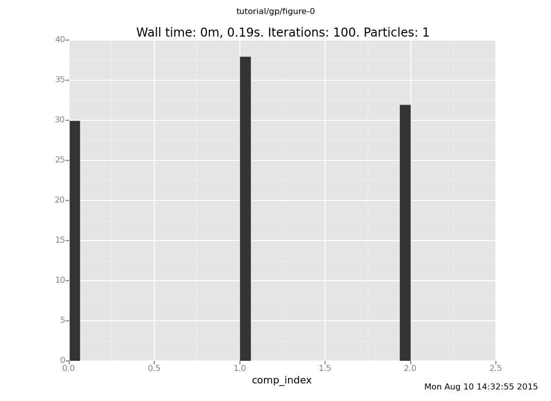
It can be instructive to examine the effect of observations. The prior on mixture components is:
plot("h0",
 run(accumulate_dataset(100,
  do(reset_to_prior,
     collect(comp_index)))))
[]
Now let's make some observations
observe mix_f() = 3.3;
observe mix_f() = 3.1;
observe mix_f() = 4.5;
and examine the posterior
plot("h0",
 run(accumulate_dataset(100,
  do(reset_to_prior,
     mh(quote(comp_index), one, 20),
     collect(comp_index)))))
[]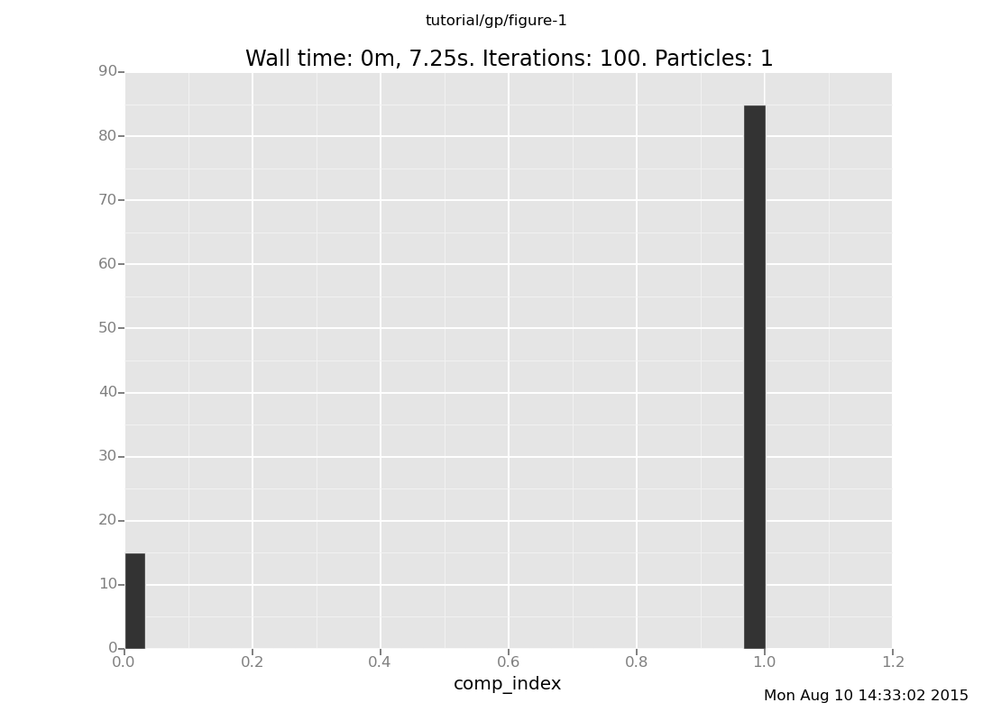
As we would expect, the possibility of uniform_continuous(0, 2) (component 2) has been
eliminated, as the sampled values of mix_f() are not possible in that component.
The remaining components are uniform_continuous(0, 10) and
uniform_continuous(0, 5).
Notice that uniform_continuous(0, 10) (component 0) is much less probable than
uniform_continuous(0, 5) (component 1) in the posterior, whereas it was equally
probable in the prior. This is a case of the Bayesian Occam's
razor: among models that agree with the data, Bayesian inference
automatically favors more parsimonious ones, because they are better
able to concentrate predictive mass. Said differently, a specific
prediction is more impressive to get confirmed.
In the present case this shows up thus: if mix_f were
uniform_continuous(0, 10), wouldn't it be a suspicious coincidence
that three independent samples of mix_f() were all between 3 and 5?
The coincidence would be much (in fact, exactly 2^(#data) times)
less suspicious if mix_f were
uniform_continuous(0, 5).
Taking the above one step further, we can use a mixture model to perform regression. Feel free to clear your session
clear
We are going to use a small plugin to make a custom plot. Download it and load it into VentureScript with
run(load_plugin("multiline_plot_plugin.py"));
[]The following code (gp-2.vnts) asks, "what is the posterior on models that are either linear or sine wave, conditioned on the given data?"
// Coefficient priors
assume a = uniform_continuous(-2, 2);
assume b = uniform_continuous(-2, 2);
assume c = uniform_continuous(-2, 2);
assume d = uniform_continuous(0, 3);
assume e = uniform_continuous(0, 2*3.14159);

// Mixture
assume components = array(
    proc(x) { a*x + b },
    proc(x) { c*sin(d*x + e) }
    );
assume weights = simplex(0.5, 0.5);
assume true_f = categorical(weights, components);

// Data (inline, in this case)
define data_xs = array(8.73, 7.47, 0.11, 0.26, 3.94, 4.86, 4.07, 5.65, 9.1, 6.62, 9.98, 3.54, 8.12, 5.17, 5.39);
define data_ys = array(0.53, 0.67, 0.23, 0.02, 0.13, 0.27, 0.33, 0.04, 0.68, 0.17, 0.1, 0.16, 0.53, 0.42, 0.4);
define data = zip(data_xs, data_ys);

// Function for programmatically observing the data
define obs = proc(xy) {
    x = lookup(xy, 0);
    y = lookup(xy, 1);
    observe(normal(true_f(unquote(x)), 1.0), y)
};
run(for_each(data, obs));

// Collect several snapshots of the progress of inference
define xs = linspace(0, 10, 200);
define yss = array_from_dataset(run(accumulate_dataset(10,
    do(mh(default, one, 50),
       collect(mapv(true_f, unquote(xs)))))));

// Plot them
plot_lines(xs, yss, data_xs, data_ys, -2, 2, 0.5, 1.0, 1.0);
[]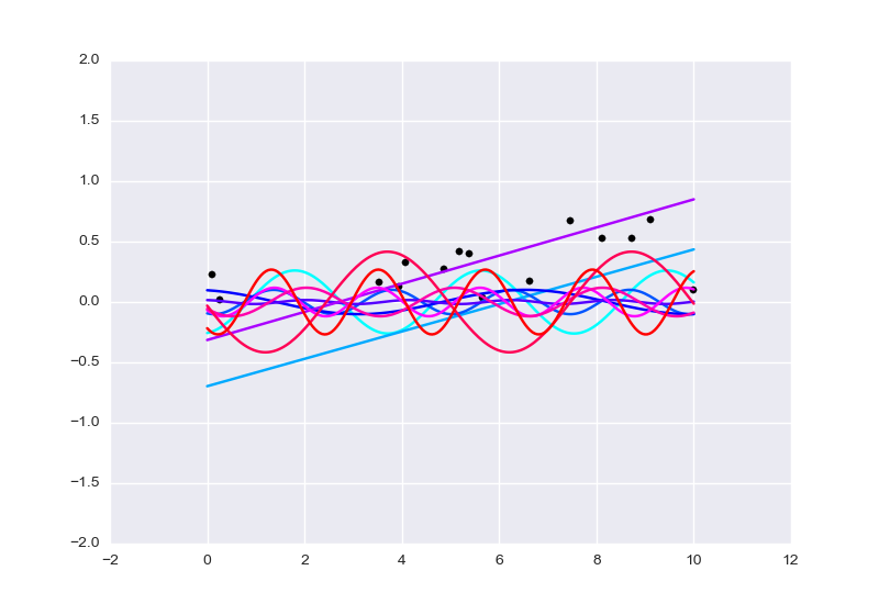
The plot contains samples of the function true_f as inference progresses, 50 steps at time. As time progresses, the hue changes from
cyan to blue to purple to red. Notice that neither a line nor a sine wave is a
perfect fit for this data set; lines incur a penalty due to the waviness of the
data and sine waves incur a penalty due to the rising pattern of the data.
(The function plot_lines(xs, yss, data_xs, data_ys, ymin, ymax, huemin,
huemax, linewidth) works as follows: scatterplot of data_xs versus
data_ys, as well as line plots of ys versus xs for each ys in yss.
As the line plots progress from the first entry of yss to the last entry of
yss, the hue of the drawn line progresses from huemin to huemax (with
hues being on a scale from 0 to 1). The lines have width linewidth, with 1
being the normal width. The plot should show up in a matplotlib window.)
Another interesting case of mixture regression is when the mixture components are models of increasing power, where more powerful models are harder to tune/fit to the data. In that case mixture regression can be viewed as a way of training all the components in parallel, and a sample of the computed (approximate) posterior consists of a choice of model along with values of the parameters for that model. We now present such an example, with observation data as shown below:
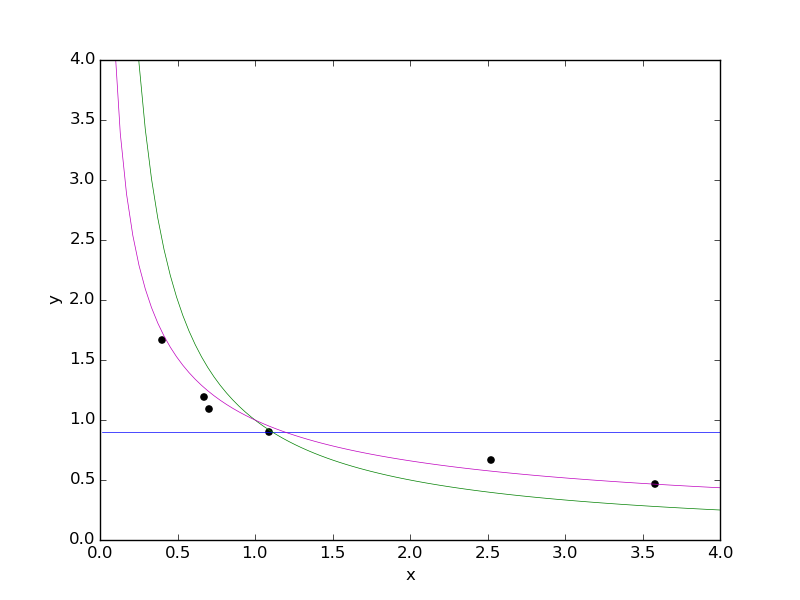
We have drawn in curves for each of the three mixture components we will be
using in our mixture model: y = 0.9 (blue), y = 1/x (green), and y = x^(-r)
(magenta, with parameter value r = 0.6). Now let's clear our session
clear
and look at a probabilistic program for regression using this mixture (gp-3.vnts):
// Parameter for component 2
assume r = tag(quote(r), 0, beta(2,2));

// Mixture
assume pcomponents = array(
    proc(x) { 0.9 },           // component 0
    proc(x) { pow(x, -1) },    // component 1
    proc(x) { pow(x, 0 - r) }  // component 2
    );
assume pweights = simplex(0.3, 0.3, 0.4);
assume pnum = tag(quote(pnum), 0, categorical(pweights));
assume pf = lookup(pcomponents, pnum);

// Data
define xs = array(0.67, 3.58, 2.52, 1.09, 0.7, 0.4);
define ys = array(1.19, 0.47, 0.67, 0.9, 1.09, 1.67);
define data = zip(xs, ys);

// Observe data points
define obs_pf = proc(xy) {
    x = lookup(xy, 0);
    y = lookup(xy, 1);
    observe(normal(pf(unquote(x)), 1.0), y)
};
run(for_each(data, obs_pf));

// Do inference, and plot the inferred values of r and pnum over time
define dataset = run(accumulate_dataset(100,
    do(if(eq(run(sample(pnum)), atom<2>)) { mh(quote(r), one, 10) } else { pass },
       mh(quote(pnum), one, 10),
       collect(pnum, r))));
plot("p0d1dcd", dataset);
[]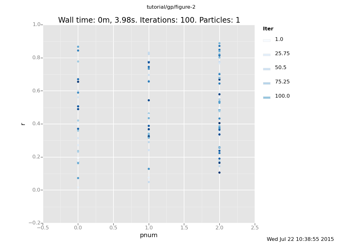
Above, the parameter r is plotted against pnum (where pnum = 0 for y =
0.3, pnum = 1 for y = 1/x, and pnum = 2 for y = x^(-r)). The darker
points correspond to later in time, i.e. after more inference steps.
Note that the inference loop contains the instruction
if(eq(run(sample(pnum)), atom<2>)) { mh(quote(r), one, 10) } else { pass }
This says, if the current value of pnum is 2 (so that y = x^(-r)), then do
inference on r, and otherwise, do not touch r. This is a sensible thing to
do since the likelihood is indifferent to r if pnum != 2, so any inference
steps taken on r when pnum != 2 would retrogress on inference progress.
Thus we see a case in which fully programmable inference is beneficial.
Subtle: It is tempting to think of inference on this mixture model as a
search: first to find the "right" component, then to find the "right"
parameters for that component. That cartoon often doesn't correctly capture
the Bayesian picture of inference. The posterior probability of a component is
the average goodness (in terms of likeilhood) of using that component with
parameters drawn randomly from the prior. So the question of whether one
particular max a-posteriori (MAP) solution will dominate the posterior depends not just on (1) how
likely the MAP solution is, but also on (2) the prior on parameters, and (3)
how wide a region of very-good solutions surround the MAP, which is related to
how sensitive the likelihood is to small changes in the parameters. In the
above example, r is the only parameter.
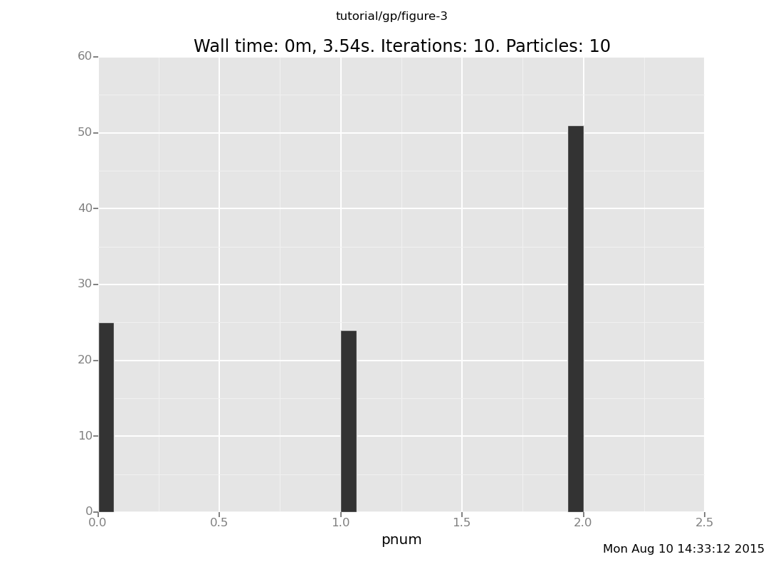
Exercise:
Compute a coarse approximation to the posterior on mixture components. Does this model make a clear choice on this data set? (show answer)
Answer:
infer resample(10);
plot("h0", run(accumulate_dataset(10,
 do(posterior,
    collect(pnum)))))
[]
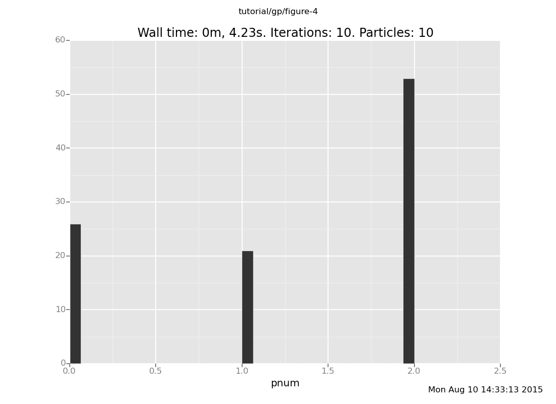
Come up with a prior on r such that component 2 (x^(-r)) dominates the
posterior.
(show answer)
Answer: Setting r to be deterministically the "right" value will
favor that component. Of course, since the "right" value
is in this case inferred from the data (by eyeballing), this risks
overfitting.
observe r = 0.6;
infer resample(10);
plot("h0", run(accumulate_dataset(10,
 do(posterior,
    collect(pnum)))))
[]
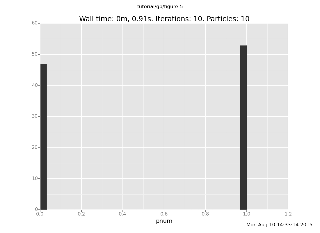
Come up with a prior on r such that component 2 is very
improbable in the posterior (but don't cheat -- the region from r = 0.4 to
r = 0.8 should still have positive probability).
(show answer)
Answer: Putting a very broad prior on r lets us produce an
arbitrarily severe Bayes Occam's Razor penalty against it.
clear
assume r = uniform_continuous(-100, 100);


// Mixture
assume pcomponents = array(
   proc(x) { 0.9 },           // component 0
   proc(x) { pow(x, -1) },    // component 1
   proc(x) { pow(x, 0 - r) }  // component 2
   );
assume pweights = simplex(0.3, 0.3, 0.4);
assume pnum = tag(quote(pnum), 0, categorical(pweights));
assume pf = lookup(pcomponents, pnum);

// Data
define xs = array(0.67, 3.58, 2.52, 1.09, 0.7, 0.4);
define ys = array(1.19, 0.47, 0.67, 0.9, 1.09, 1.67);
define data = zip(xs, ys);

// Observe data points
define obs_pf = proc(xy) {
   x = lookup(xy, 0);
   y = lookup(xy, 1);
   observe(normal(pf(unquote(x)), 1.0), y)
};
run(for_each(data, obs_pf));


infer resample(10);
plot("h0", run(accumulate_dataset(10,
 do(posterior,
    collect(pnum)))))
[]
(Open ended) What other parts or aspects of the model have a describable effect on the behavior of inference?
While the above examples rergess nonlinearly on a data set, the mixture components are still hard-coded parametric models, and as such, the amount of modeller/programmer resources required to write them grows with the complexity of the model.
We will now look at Gaussian process models, which "let the data speak for itself" in the sense that the "effective dimensionality" of the model grows with the number of data points. For an introduction to Gaussian processes viewed as random functions, see Section 2.2 of Rasmussen and Williams.
clear
This segment requires a more elaborate plugin, where we implement a Gaussian process as a foreign stochastic procedure. Load it with
run(load_plugin("multiline_plot_plugin.py"));
run(load_plugin("gpexample_plugin.py"));
[]and set up the Gaussian process like so
// Covariance function
assume se = make_squaredexp(1.2, 0.8);

// Mean function
assume zero_func = make_const_func(0.0);

// Gaussian process
assume g = make_gp(zero_func, se);
<venture.lite.gp.GP object at 0x2b091fe2f9d0>The Gaussian process g can be thought of as a random function whose prior is
a Gaussian process with mean zero and covariance function se, that is,
squared exponential:
prior_covariance(g(x1), g(x2)) = 1.2 * exp((x1-x2)^2 / (2*0.8))
We can observe the value of g at given data points:
// Data
assume data_xs = array(3.2, 2.2, 8.7);
define data_ys = array(8.7, 0.2, 5.5);
infer observe(g(data_xs), data_ys);

// Plot several samples of the gp
define xs = linspace(0, 10, 200);
define yss = mapv(proc(i) {
    run(sample(g(unquote(xs))))
}, arange(10));
plot_lines(xs, yss, run(sample(data_xs)), data_ys, -5, 12, 1.0, 1.0, 0.5);
[]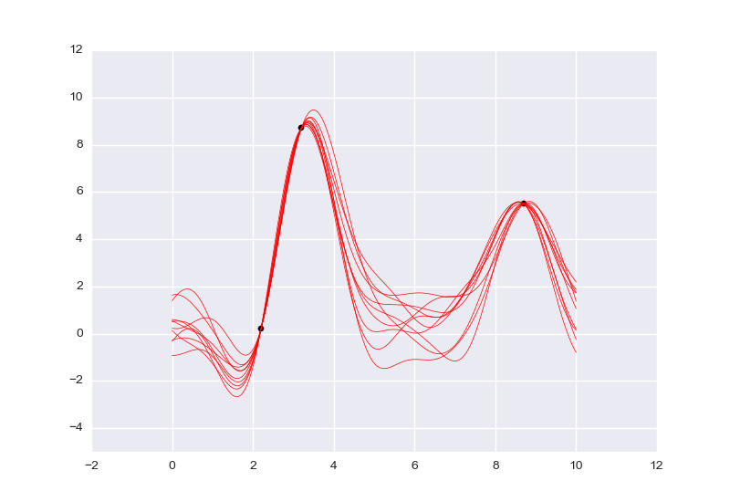
(The above two VentureScript blocks are gp-4.vnts.)
The posterior of g is again a Gaussian process (several samples of which are
plotted above), with a different mean function and a different covariance
function (see R&W for
more on this). The inputs and outputs of g are arrays, because g samples
from the joint distribution of the GP's values on all supplied inputs.
Exercise: Consider the following three ways to query a GP.
// Way 1
sample g(array(1.0, 2.0));

// Way 2
sample g(1.0);
sample g(2.0);

// Way 3
sample array(g(1.0), g(2.0));
[-2.615749041146829, -1.1918682496288109]Ascertain the distributions on values they produce. Are they the same or different? (show answer)
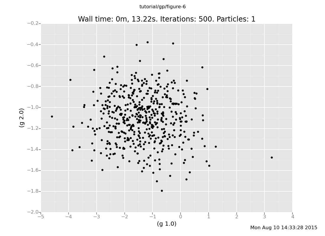
Answer: Here's the distribution given by Way 2:
plot("p0d1d", run(accumulate_dataset(500, collect(g(1.0), g(2.0)))))
[]
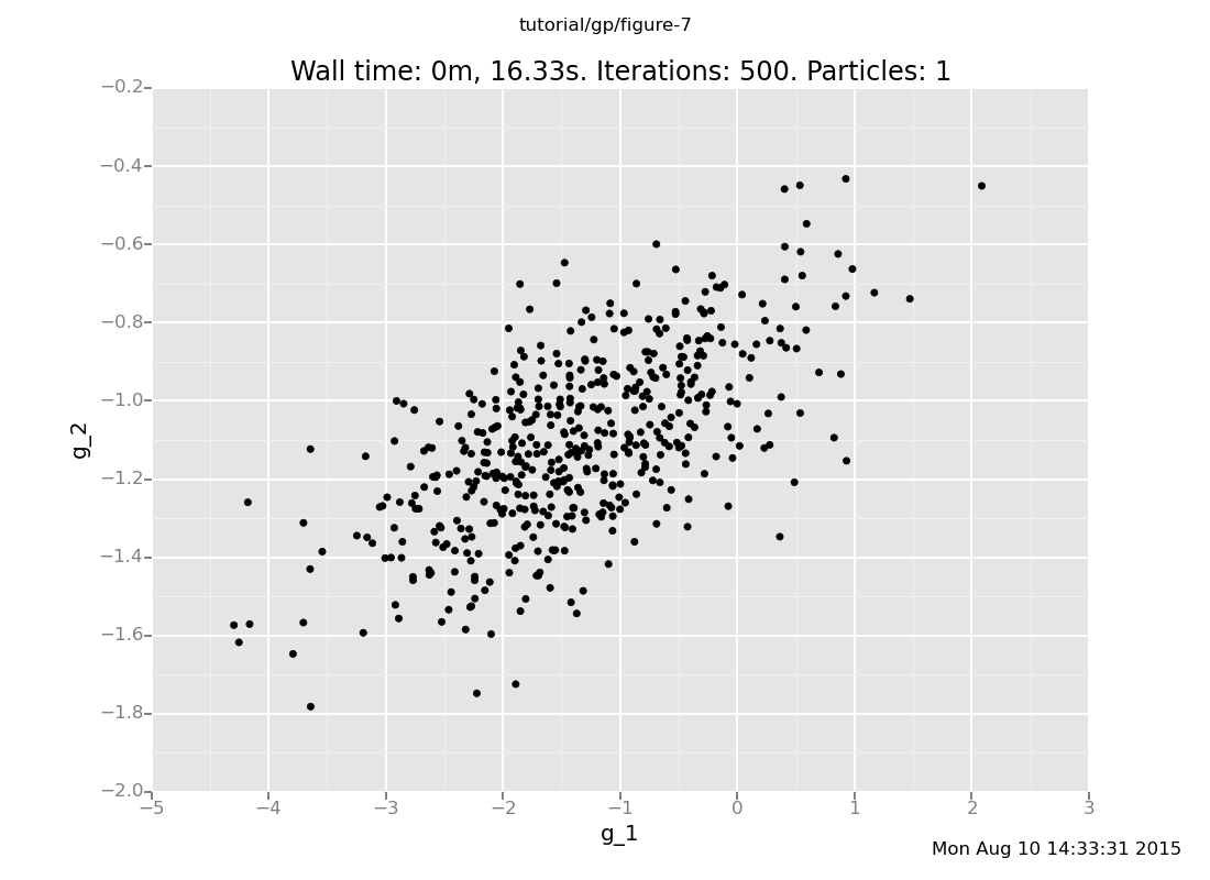
Plotting Ways 1 and 3 is a little trickier, because collect doesn't
(yet) have native support for vector-valued expressions (the use of
labelled is needed to align the data):
plot("p0d1d", run(accumulate_dataset(500,
 do(vals <- sample(array(g(1.0), g(2.0))),
    collect(labelled(lookup(quote(unquote(vals)), 0), g_1),
            labelled(lookup(quote(unquote(vals)), 1), g_2))))))
[]
plot("p0d1d", run(accumulate_dataset(500,
 do(vals <- sample(g(array(1.0, 2.0))),
    collect(labelled(lookup(quote(unquote(vals)), 0), g_1),
            labelled(lookup(quote(unquote(vals)), 1), g_2))))))
[]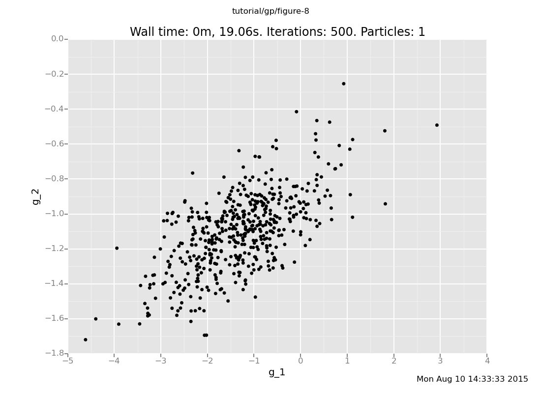
Ways 1 and 3 produce the same multivariate Gaussian, whereas Way 2 produces independent samples.
Why does that happen? (show answer)
Answer: Let's take them one at a time.
Way 1 is the "right" way to query a Gaussian process: supply all the test inputs at once. By definition, the GP returns a sample from a multivariate Gaussian determined by the mean and covariance functions applied to those points and previously queried ones.
Way 2 exhibits an important property of VentureScript: a sample
expression does not modify the model. So, the GP cannot "remember"
the value sampled at x=1.0 when sampling at x=2.0, and produces
independent samples.
Way 3 is "right" again. Expressions evaluated in the same sample
command can influence each other. Way 3 samples a value from the
GP at x=1.0 conditioned on the observations, and then one at
x=2.0 conditioned on the observations and the value at x=1.0.
Note that the choice of covariance function can itself be random (as long as
all possible functions are symmetric and positive-semidefinite). For example,
rather than defining se = make_squaredexp(1.2, 0.8), we could have defined
se = make_squaredexp(sigma_prior(), l_prior()), where sigma_prior and
l_prior are stochastic procedures. The inference engine could then be used
to perform parameter estimation; in fact, we do this below, in the section on
Bayesian optimization. It would even be possible to infer the structure of the
covariance function, if we had in mind a generative model of covariance
function structures.
In this segment, we will play with a new idiom for GP modeling
that the Venture team recently developed language support for, called
Gaussian process memoization, or gpmem. The idea is to wrap a function f
into a package containing both a self-caching "prober" (which actually calls
f) and a statistical emulator, which simulates f using a GP prior
conditioned on the values of all previous invocations of the prober. The
arguments to gpmem are the function f, a prior mean function for the
GP-based emulator, and a prior covariance function. For example (gp-5.vnts):
clear
run(load_plugin("gpexample_plugin.py"));

// Function to model
assume f = make_audited_expensive_function("f");

// Mean and covariance functions for the GP emulator
assume zero_func = make_const_func(0.0);
assume se = make_squaredexp(1.2, 0.8);

// GPMem package
assume package = gpmem(f, zero_func, se);

// Test
assume ffive = first(package)(5);
assume fsix = first(package)(6);

sample second(package)(array(5.5))
[PROBE f] Probe #1: f(5.000000) = -0.391519
[PROBE f] Probe #2: f(6.000000) = -0.641769
[-0.42951469]Note that the emulator expects an array as input (since it is a GP, as above),
but the prober does not (since f is just a function, there is no need to
"jointly" evaluate f at multiple points).
Our original motivation for this idiom was the case when f is too expensive
to compute many times, so we need to learn using a limited number of samples.
Later we realized that GP regression in general can be cast as a special case
of gpmem: regression on a dataset D (with keys x and values y = D[x])
is the same as statistical emulation of the function f defined in pseudocode
as
def f(x):
  if x in D:
    return D[x]
  else:
    raise Exception("Illegal input")
Observing data points {(x, y)} is the same as probing the value of f at all
the xs.
If you can think of any other potential applications of gpmem, we would love
to hear them.
The example below showcases several nice features of gpmem and GP modeling
in VentureScript. In the code below we aim to find the maximum value of our
expensive function V on the interval [-20, 20] using as few evaluations of
V as possible. We do this by wrapping V in a gpmem and repeatedly using
the GP-based emulator to find a point where we have the most evidence than V
will be large. We probe V at said point, which gives our GP model more
information to choose the next probe point. In addition, we perform
Metropolis-Hastings inference on the hyperparameters of the covariance function
after each probe (gp-6.vnts).
clear
run(load_plugin("gpexample_plugin.py"));

// The target
assume V = make_audited_expensive_function("V");

// The GP memoizer
assume zero_func = make_const_func(0.0);
assume V_sf = tag(quote(hyper), 0, uniform_continuous(0, 10));
assume V_l = tag(quote(hyper), 1, uniform_continuous(0, 10));
assume V_se = make_squaredexp(V_sf, V_l);
assume V_package = gpmem(V, zero_func, V_se);

// A very naive estimate of the argmax of the given function
define mc_argmax = proc(func) {
  candidate_xs = mapv(proc(i) {uniform_continuous(-20, 20)},
                      arange(20));
  candidate_ys = mapv(func, candidate_xs);
  lookup(candidate_xs, argmax_of_array(candidate_ys))
};

// Shortcut to sample the emulator at a single point without packing
// and unpacking arrays
define V_emu_pointwise = proc(x) {
    run(sample(lookup(second(V_package)(array(unquote(x))), 0)))
};

// Main inference loop
infer repeat(15, do(pass,
    // Probe V at the point mc_argmax(V_emu_pointwise)
    predict(first(V_package)(unquote(mc_argmax(V_emu_pointwise)))),
    // Infer hyperparameters
    mh(quote(hyper), one, 50)));
[PROBE V] Probe #1: V(-18.440282) = 0.151536
[PROBE V] Probe #2: V(-2.517947) = 0.446890
[PROBE V] Probe #3: V(-3.177060) = 0.235179
[PROBE V] Probe #4: V(18.686960) = 0.143810
[PROBE V] Probe #5: V(-0.337970) = 0.982476
[PROBE V] Probe #6: V(0.425688) = 1.039088
[PROBE V] Probe #7: V(13.013558) = 0.251995
[PROBE V] Probe #8: V(-1.300065) = 0.797444
[PROBE V] Probe #9: V(1.872153) = 0.869653
[PROBE V] Probe #10: V(0.868096) = 1.027747
[PROBE V] Probe #11: V(-0.195912) = 0.999769
[PROBE V] Probe #12: V(-13.625254) = 0.275500
[PROBE V] Probe #13: V(-19.864960) = -0.028693
[PROBE V] Probe #14: V(11.368950) = -0.097100
[PROBE V] Probe #15: V(0.433885) = 1.039187
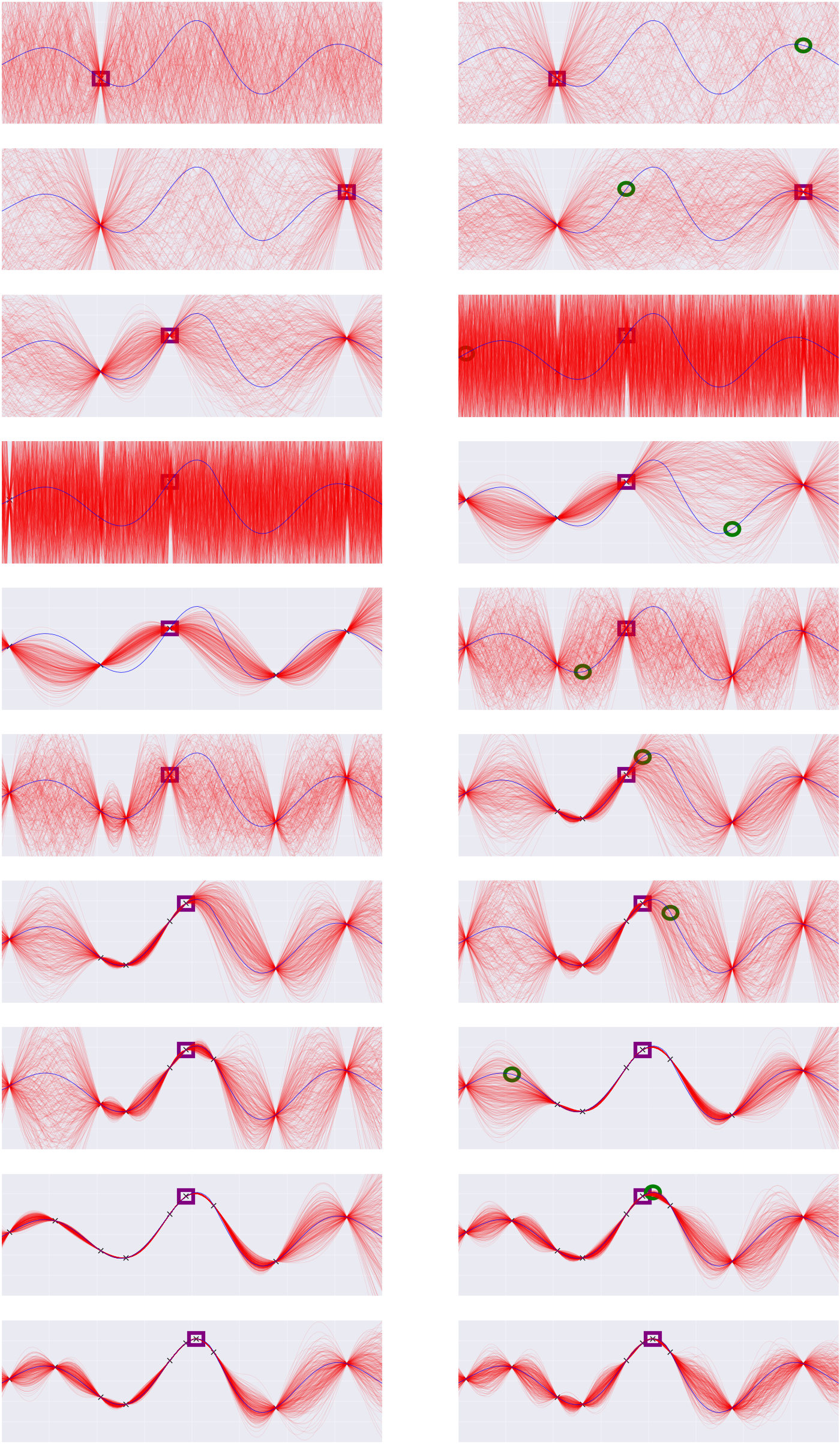
[]Here is a visualization of a run of this program (not the same run as above),
showing the state of the emulator at various times. Each row adds a new probe
point. The left column is before hyperparameter inference, the right column
after. The blue curve is the true function V, the green circle is the next
chosen probe point, and the purple square is the best probe point found so far.
Notice that probes tend to be chosen either where the value of the emulator is
high, or where the emulator has high uncertainty. Also note that the "crazy"
plots on the third-fourth rows correspond to a "crazy" choice of parameters.
This is not a mistake -- Metropolis-Hastings samplers will make crazy choices
every once in a while (as will the true posterior, with some small
probability).
| < Prev: More VentureScript: Linear Regression | ^ Top |